
Introduction
I regularly get questions on using solar panels to power our Fiber-To-The-Home gear (FTTH). You might think that sounds kind of odd, but it makes a lot of sense for many businesses and municipalities. For example, every municipality has water towers, sewage lift stations, and energy delivery systems that have alarm sensors that need to be monitored. In the old days, phone lines could be used to provide both connectivity and power to these sensors (e.g. powered T1 lines). However, FTTH systems are connected with glass and there is no way to provide any electrical power down these lines. Businesses also have remote pipelines and electrical distribution systems with sensors that need to be monitored. I even had one ranch that wanted to provide voice, video, and data services to a remote bunkhouse for cowboys. Many businesses want to take advantage of solar energy because it contributes to the lessening of greenhouse emissions on Earth, helping to reduce global warming and climate change. Businesses could look at Reliant Energy reviews which could assist in finding the best price for solar energy production if they were interested in getting solar panels.
As with any power system, you want to get the maximum amount of power possible out of a solar panel. As with most electrical systems, solar panels put out the most power when they are presented with an optimal load. Figure 1 shows an example of the current versus voltage curves (aka "i-v curves") for a typical solar panel (Source). The i-v curves are represented by the solid lines and the available power is represented by the dashed lines.

Figure 1: Photovoltaic Current versus Voltage Curves.
To get optimum power from a solar panel, the load presented to the solar panel must be varied as the incident solar power varies through the day. Fortunately, switching power supplies allow us the vary the input load while maintaining they maintain a constant output voltage, which is important for doing things like charging batteries.
Ideally, we would have a circuit that would allow us to monitor the power output from the solar panel and would vary the switching power supply load as needed to achieve optimum results. It turns out there are a number of ways to accomplish this feat, which is called Maximum Power Point Tracking (MPPT). While investigating various MPPT designs, I encountered the following article by Stephen Woodward. I always admire Woodward's designs – they are elegance writ in silicon. I will not review his entire circuit, rather I will examine how he computes the power from the solar panel using very simple electronics.
Background
Approach
Most MPPT controllers use a perturbation-based approach to determine the optimum load they need to present. In general, they deliberately create a small load disturbance to the solar panel and they determine whether power increased or decreased. They will change their load to ensure that they are constantly adjusting their load to increase the power from the solar panel. Generally, these schemes compute power by multiplying the current value by the voltage value. This approach often requires analog multipliers (expensive) or software (demands software, memory, and a processor – also expensive). This approach assumes that we can compute the power from the solar panel. Woodward's design includes a beautifully simple means for generating a voltage that is related to power. Maximizing this voltage will also maximize the power we obtain from the solar panel.
Woodward's Solution
It is well known that the voltage across the base-emitter junction can be described by Equation 1.
| Eq. 1 | 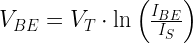 |
where
- VBE is the base-emitter voltage of the transistor.
- IBE is the base-emitter current of the transistor.
- IS is the saturation current of the transistor (it varies from device to device).
- VT is the thermal voltage
from the Shockley equation.
Figure 2 illustrates the accuracy of this relation with respect to an actual transistor (2N3904). This plot shows base-emitter voltage versus collector current. Collector current is closely related to the base-emitter current by the equation 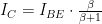
.")
Figure 2: Semilog Plot of a 2N3904 Transistor (Typical NPN Device).
Woodward's approach is simple:
- Note that
. Since maximizing the logarithm of the power is the same as maximizing the power, we can maximize this equation and obtain our objective.
- Use two cheap, identical transistors in series.
- Drive one of the transistor with a current proportional to the voltage from the solar panel.
- Drive the second transistor with a current proportional to the current from the solar panel.
- Since the transistors are in series, their voltages sum will be the related to the logarithm of the product of solar panel current and voltage, i.e. power.
Circuit
Woodward's original contained the multiplier sub-circuit shown in Figure 3. As mentioned earlier, the sum of the Q1 and Q2 Collector-Emitter (CE) voltages represent the power being drawn from the solar panel.

Figure 3: Schematic of Woodward's Analog Multiplier.
VSum represents the logarithm of the power and is used to optimize the power transfer. Note that the emitter of Q2 is at virtual ground.
To analyze this circuit, let's break it down into two parts: (1) the CE voltage for Q1 (VQ1), and (2) the CE voltage for Q2 (VQ1).
Transistor Q1 Voltage
Figure 4 shows the circuit used to generate a current proportional to the solar panel voltage, which then produces a voltage across Q1. Amplifier A2 is used to build a negative resistor. As shown in Figure 4, this negative resistor, when combined with the solar panel voltage (VPV) and R1, is used to build a current source that produces 

Figure 4: Schematic of Circuit Section that Generates A Q1 Current Proportional to the PV Voltage.
This current means that the CE voltage of Q1 can be written as
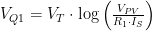 .
.
Transistor Q2 Voltage
Figure 5 shows how Q2's voltage is generated. Amplifier A1 is used to build a current source that draws 
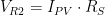

Figure 5: Schematic of Circuit Section that Generates A Q2 Current Proportional to the PV Current.
This current means that the CE voltage of Q2 can be written as
 .
.
Voltage Sum
Equation 2 gives us the voltage across Q1 and Q2.
| Eq. 2 |  |
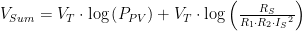 |
where 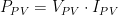
Thus, we can maximize the power obtained from the solar panel by maximizing the voltage given by Equation 2.
Conclusion
This circuit nicely illustrates how the clever use of the logarithmic characteristic for a transistor junction can be used to make a simple and inexpensive power calculation circuit. In a later post, I will show how this circuit can be combined with a switching power supply to make an MPPT controller for a solar panel.
Update
Another engineer beat me to it. See this blog post. It references this post and includes a complete design for an MPPT controller.
Hi I like you post make me understand better. I am looking forward to see the MPPT controller for a solar panel.
If you build an MPPT controller, send me a note. I like to see what people are building.
mathscinotes
Another engineer has now designed a complete MPPT with this circuit. See this blog.
http://www.ko4bb.com/Solar_Optimizer/
Mathscinotes
Pingback: Powering Telecom Gear Using Energy Scavenging | Math Encounters Blog
Pingback: MPPT bez mikrokontrolera / MPPT without microcontroller | DareIT
Pingback: Top 94 cross-modulation Things You Should Know – CLOUDCOMPUTINGSURVIVAL.COM