Some Laser Basics

Introduction

I am doing some interesting work with lasers this week. I thought it would be useful to provide some background on how we build and control lasers. We deploy a lot of lasers in outdoor applications, which means that special attention must be paid to the temperature characteristics of lasers. If you are a small business that is considering getting a laser cutter then you should probably do your research to understand better how laser cutters work, you could take a look at something like this best laser cutter for small business to show you what could be offered to you. Keep on reading though to find out more about lasers, the automotive supply chain and how they work. Like batteries, lasers have characteristics that vary with temperature, with some industrial lasers needing products like North Slope needed to mitigate the heat and stabilize equipment for optimal laser performance. These temperature variations would cause the laser's output power to drop if actions were not taken to compensate for the temperature variations. These variations also make a laser subject to thermal runaway, also just like a battery. This week's work will focus on temperature compensation. But first, let's discuss how our lasers operate and are assembled. Once we have established that base, we can move on to related topics.

Laser Basics

Lasers emit light when they are driven by current above a level called the threshold current (symbolically I_Threshold). The more current you drive into the laser above the threshold level, the more optical power that the laser emits. Figure 1 illustrates this characteristic.

Figure 1: Idealized Laser Output Power Versus Input Current Characteristic.

Let's summarize the key points of Figure 1:

• No optical power is emitted until the drive current exceeds a given value called I_Threshold.
• For drive currents above threshold, the laser emits an optical power proportional to the amount that the drive current exceeds the threshold level
• The constant of proportionality is called Slope Efficiency (SE)

We can model this characteristic using Equation 1.

Eq. 1

This power versus drive current characteristic by itself does not cause any problems. However, I_Threshold and SE both vary with temperature and this is the source of my woes. Figure 2 shows how the laser characteristics vary with temperature for a real device. Notice how the slope efficiency reduces with increasing temperature. That is the key problem, as I will discuss below.

Figure 2: Slope Efficiency Graph for an Actual Laser.

Controlling Laser Power

Communication Using Lasers

Digital communications using fiber optics is similar to many other forms of digital communications in that we encode binary information by sending light down the fiber at two different power levels. The high-level is called a "1" and the low-level is called a "0". Figure 3 illustrates what an idealized optical bit stream looks like.

Figure 3: Example of a Digital Bit Stream Using Optical Power Modulation.

Because SE decreases with temperature, maintaining constant "1" and "0" levels means increasing the drive current with increasing temperature. It turns out that this is a more difficult problem to solve than you might think. Figure 4 shows how we convert drive current into optical power. We try to control two parameters:

• I_Bias, which controls the average power level
• I_Modulation, which controls the difference between P₀ and P₁.

Figure 4: Conversion of Drive Current Into Optical Output Power.

Over the years, we have used various temperature compensation techniques. It turns out that controlling a laser's output power near room temperature is simple. However, particularly at high temperature, problems develop because the drive current becomes so high that the laser self-heats. This self-heating results in lower SE, which means more drive current. The laser is now in thermal runaway, which means our control circuitry will need to shut down the laser to prevent damage.

We have used feedback to control the laser's average output power 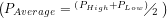. However, controlling the average power is not sufficient. Receivers actually detect the difference in power between a "1" and a "0". Reduced SE also reduces the difference between a "1" and "0". So we need an approach that will both increase the difference between the "1" and "0" drive levels and maintain an average power setting.

We have used a mathematical model for the variation of SE with temperature and have used this model to predict the required increase in the difference between the "1" and "0" drive levels with temperature. This has proven to be a mediocre solution. The temperature characteristics of a laser vary by vendor and lot. We need something better -- we need a two feedback loops. One feedback loop to control average power and another to control the difference in levels between a "1" and "0". It turns out that a new "dual-loop" laser drivers are now becoming available. Future posts will discuss how these devices work.

Basic Laser Construction

Before I go too far into controlling a laser, let's talk about how commercial laser systems are constructed. Figure 5 illustrates how lasers are typically configured for use in communications applications. The laser is mounted so that the vast majority of the optical power generated goes into the fiber, with a tiny fixed percentage tapped off for measurement by a photodiode (called the monitor photodiode). In Figure 2, the light going to the left is focused into fiber by some type of lens, which is commonly a ball lens but can be other types.

Figure 5: Standard Laser Configuration for Communications Applications.

Figure 6 shows how lasers are packaged into transistor-outline (TO) cans, which is how we often see them.

Figure 6: Illustration of Laser TO-Can Packaging.

Conclusion

This post was intended to provide some background for the posts to follow. These posts will look at applying lasers in communications applications.