
Quote of the Day
Policy is an illustration of character.
— Dick Morris, political analyst. While this quote was stated in a political context, it also holds true for engineering management.
Introduction

Figure 1: CWDM Wavelength Grid. (Source)
Nothing like reading ITU optical specifications to help you get to sleep after an active day. Since I have been doing some work on dispersion, let's pull up ITU G.695 - Characteristics of Optical Systems. I want to see if the work published in my previous blog posts on dispersion are consistent with what is contained in an industry standard. This will be a fairly brief post, but it will pull together the information from several previous posts.
Background
Coarse Wavelength Division Multiplexing (CWDM) Review
Engineers often put multiple wavelengths (i.e. colors) on a single fiber in order to to increase the amount of data that we can carry (Figure 1). The ITU has defined some standard wavelengths that everyone has agreed to use. Some of these wavelengths are listed in Figure 2. Fiber has a different level of dispersion for each wavelength. I will perform the dispersion calculations for the eight wavelengths that I am interested in.

Figure 2: Table from ITU G.694 Showing Standard CWDM Wavelengths.
Dispersion Background
I have written about dispersion in two sets of posts:
I will show that here some of the data in ITU G.695 can be generated using the information in these posts. This topic came up in an email chain last week and I thought I write down the gist of that discussion.
Analysis
Dispersion Power Penalty Formulas
For limited amount of dispersion (< 3 dB), we can model dispersion as a loss of optical power. This allows dispersion to be modeled in the same way as attenuation and connector losses. In one of my previous posts, I gave three formulas that were fundamentally different (a fourth formula presented was just an approximation to one of the other three). I repeat the formulas here as Equations 1 through 3.
| Eq. 1 | 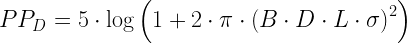 |
| Eq. 2 | 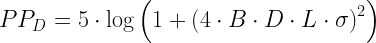 |
| Eq. 3 |  |
where
- B is the bit rate
- L is fiber distance.
- D is the dispersion constant of the fiber
is the spectral width of the laser
Note how each equation contains the product B∙D∙L∙σ, which I will refer to as the dispersion product. This product is the key to understanding how the G.695 specifications for dispersion were generated.
Discussion of the Dispersion Product
Equation 4 shows how we can think of the dispersion product as being composed of two terms determined by different aspects of the system: (1) a fiber plant-dependent term, and (2) a transmitter-dependent term.
| Eq. 4 | 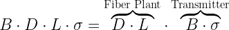 |
The role of the standard is to state achievable fiber plant characteristics (i.e. D·L) for which the optical manufacturers can develop interoperable optical product designs, which are can control B·σ.
Determination of the Fiber Plant Term
The specific case that I am worried about uses Corning SMF-28e fiber, which complies with ITU G.652, over an 80 km distance. This means that I can compute the fiber plant term as shown in Figure 3.

Figure 3: Computation of the Fiber Plant Term for a 10Gbps, 80 km Fiber Link.
ITU Assumptions for D(λ)
An industry standard has to be written so that its requirements can be met by the vast majority of manufacturers. In the case of ITU G.652, they layout their assumptions for D(λ). We can use the result of this blog post to see how the SMF-28e's D(λ) data relates to the industry standard's D(λ) assumptions (Figure 4).
.")
Figure 4: Comparison of G.652 and SMF-28e Value for D(λ).
Dispersion Power Penalty and G.695
When you look at the optics specifications for a 10 Gbps(gigbit per second) transmitter rated for 80 km, they usually assume a 1300 ps/nm dispersion "load" for test purposes. Figure 5 shows the range of power penalties we should expect to see for this optics.

Figure 5: An Example of the Dispersion Calculations.
These are all reasonable values for a high-end network.
Conclusion
Applying a bit of theory, I was able to reconstruct a few of the specifications from G.695 that we will be using in our work. This means that I understand what the critical parameters in the dispersion problem are and I can feel confident in moving forward -- and go to sleep.