Rule of Thumb for Wood Shrinkage

Introduction

As winter comes, I often see homes where gaps develop in the wood flooring, molding, or ceilings (Figure 1) – things are drying out. While I have never actually spent any time investigating the mechanism of wood's movement or magnitude, I see its effects all the time.

Figure 1: Examples of Seasonal Wood Movement.

Source	Source	Source

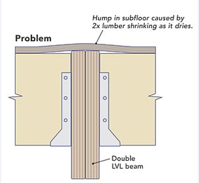
Recently, I read a forum discussion in Fine Homebuilding magazine that got me interested in working through a numerical example of wood movement. The article did a great job explaining how a wood floor can develop a "bump" in it (Figure 2, left) and the simple remedy of setting the joists a bit lower (Figure 2, right) to prevent the joist from poking through. This drawing explains the occasional bumps in flooring I have encountered in new homes (i.e. ones with LVL beams). The key issue is that engineered beams and standard dimensional lumber beams have different expansion/contraction characteristics – dimensional lumber moves much more.

Figure 2: Fine Homebuilding Explanation For a Seasonal Floor Bump and the Fix.

My objective in this post is to understand how moisture affects wood, with respect to its physical dimensions. Whilst many have found that looking to check out the floor sanding and polishing options available by leading floor sanding companies on this page helps them keep this in check, there are other measures that should be considered long before this. Since I like to focus on a specific problem to drive my inquiry, I have decided to verify a rule of thumb from the Fine Homebuilding article mentioned above. The rule of thumb is:

By checking the moisture content of the lumber before it's installed, framers can predict the amount of movement that will occur across the grain of dimensional lumber. It's not an exact science, but a good rule of thumb is that if the moisture content of a board changes by 4%, the board will shrink across the grain by approximately 1% of its width. You may need termite control los angeles services called in as some people experience termites in their furniture if there is any water damage or if a large amount of moisture comes into contact. If you have water damage it is a good idea to contact a service like ServiceMaster Restoration by Zaba to help before the problem gets worse. And getting rid of the furniture is all well and good, but you want to stop this from affecting anything else within the house. This is why it may be best to look into something like Termite Control Kansas City to help return your property back to its original state. Tho/blockquote>
I will take a quick look at this rule of thumb and see if I can explain how it was derived. I also derive a relationship between two common formulas used to estimate the movement of wood and the coefficients used in these formulas for the different species.

Background

Some Definitions

Moisture In Wood

The following definitions all refer to Figure 3. The information here comes from this web page, which I strongly encourage you to visit.

Figure 3: Section Drawing of Wood Structure.

Bound Water

Water is this hydrogen bonded to the cellulose of the wood cells.

Free Water

The water filling the wood cell cavities. For more details on these cavities, refer to the Wikipedia on xylem and phloem.

Fiber Saturation Point (FSP)

The wood moisture content level at which all the free water is gone, but the bound water is still present. We usually assume that the number is 30%, but the number actually varies with temperature and species of tree. For example, the Wikipedia states that the $FSP=0.30-0.001\cdot (T-20)$ , where T is the wood temperature.

Moisture Content (MC)

The percentage of wood mass consisting of water. It is often measured in the field using electrical test equipment (example). In the lab, it can be measured using by measuring the mass of a test sample before and after drying and computing $MC\triangleq \frac{{{m}_{water}}}{{{m}_{dry}}}=\frac{{{m}_{wet}}-{{m}_{dry}}}{{{m}_{dry}}}$ , where

m_water is the mass of water in the wood sample

m_wet is the mass of the wood sample before drying

m_dry is the mass of the dried wood sample.

Directions in Wood

Wood literally has a grain (aka growth ring) to it and the amount of movement varies with respect to the gain. Figure 4 illustrates the three directions in which wood's expansion are usually specified.

Figure 4: Illustration of Moisture-Driven, Growth Directions (from J Gibson McIlvain).

Tangential Direction

Wood movement along the growth ring, which is the direction of greatest movement.

Radial Direction

Wood movement perpendicular to the growth rings. Expansion in this direction is often smaller than in the tangential direction by a factor of 2 to 5.

Longitudinal Direction

Wood movement parallel to the grain of the wood (i.e. up and down for a standing tree). This is usually a small number (0.1% to 0.3%) and often ignored (source).

Types of Lumber Cut

Figure 5 shows the best drawing I could find of the types of saw cuts and how they change dimensionally with moisture variation. You can see why the different cuts expand differently if you visualize the wood expanding the most in the direction along the grain. I do find it interesting that the quarter sawn wood expands in thickness rather than width – this explains why I have had better luck with it in certain applications than others with respect to expansion.

Figure 5: Cut Types and How They Change Dimensionally (from Popular Woodworking).

Modeling Shrinkage

For modeling purposes, the relationship between MC and FSP controls how wood expands or contracts:

MC ? FSP, have no impact on the physical and mechanical properties of wood.
The additional water is filling up the air voids within the wood and it is not causing any dimensional changes.

MC < FSP, does impact on the physical and mechanical properties of wood.
The additional water is filling up the air voids within the wood and it is not causing any dimensional changes.

In actual fact, the transition is a bit more subtle than implied by this simple model. The following quote from Wood Handbook does a good job describing what happens. Note that the Wood Handbook uses MC_fs instead of FSP for the Fiber Saturation Point.

Moisture can exist in wood as free water (liquid water or water vapor in cell lumina and cavities) or as bound water (held by intermolecular attraction within cell walls). The moisture content at which only the cell walls are completely saturated (all bound water) but no water exists in cell lumina is called the fiber saturation point, MC_fs [FSP]. Operationally, the fiber saturation point is considered as that moisture content above which the physical and mechanical properties of wood do not change as a function of moisture content. The fiber saturation point of wood averages about 30% moisture content, but in individual species and individual pieces of wood it can vary by several percentage points from that value.

Conceptually, fiber saturation distinguishes between the two ways water is held in wood. However, in actuality, a more gradual transition occurs between bound and free water near the fiber saturation point. Within a piece of wood, in one portion all cell lumina may be empty and the cell walls partially dried, while in another part of the same piece, cell walls may be saturated and lumina partially or completely filled with water. Even within a single cell, the cell wall may begin to dry before all water has left the lumen of that same cell.

I should note that while I will focus in this post the on the dimensional changes in the width and thickness of a rectangular board, shrinkage can appear to change the angle of wood joints that are not 90°. This is because the width of wood along these joints vary, which means that the amount of shrinkage varies along the joint. See Appendix B for more details.

Analysis

Model

There are two equations that are commonly used to model the movement of wood as a function of moisture content. I will review them both here.

Equation 1 is used to model the dimensional changes when the wood's moisture content changes from 6% to 14%.

Eq. 1 $\displaystyle \delta=\left\{ \begin{array}{*{35}{l}} {{D}_{I}}\cdot {{C}_{R}}\cdot \left( {{M}_{F}}-{{M}_{I}} \right) & \text{Tangential Direction} \\ {{D}_{I}}\cdot {{C}_{T}}\cdot \left( {{M}_{F}}-{{M}_{I}} \right) & \text{Radial Direction} \\ \end{array} \right.$

where

? is the change in dimension.

D_I is the initial dimension.

C_T is tangential change coefficient.

C_R is radial change coefficient.

M_F is the final moisture content (%).

M_I is the initial moisture content (%).

For a more detailed discussion of Equation 1, see chapter 12 of the Wood Handbook (Equation 12-2). I am not going to spend much time analyzing this result because it is just a linear approximation – everything is linear if you restrict the dynamic range (i.e. range of application) sufficiently.

When the moisture change is outside the range of 6% to 14%, Equation 2 is used.

Eq. 2 $\displaystyle \delta =\frac{{{D}_{I}}\cdot \left( {{M}_{F}}-{{M}_{I}} \right)}{\frac{30\cdot 100}{{{S}_{T or R}}}-30+{{M}_{I}}}$

where

S_T is the tangential change coefficient for wood going from green to an oven-dry state (see Wood Handbook, Chapter 3, Table 3-5)

S_R is the radial change coefficient for wood going from green to an oven-dry state (see Wood Handbook, Chapter 3, Table 3-5).

For a derivation of Equation 2, see Appendix A. I have not seen many examples of Equation 2 being used by woodworking practitioners. I cover it here because it is mentioned in the Wood Handbook, but most examples use Equation 1. I assume this is true because most wood is used in applications where its moisture content does not vary outside the range of 6 % to 14 %.

While Equations 1 and 2 use different sets of coefficients, it turns out that there is a relationship between these coefficients for many species (I have not checked them all out). Appendix C goes into the gory details.

Rule of Thumb Verification

I am going to make the following assumptions:

The rule of thumb uses Equation 1 because it is applicable to the typical range for the MC of wood under normal conditions.

The rule of thumb will use the tangential change coefficient C_T because it is the largest coefficient, which means that the rule of thumb gives a worst-case estimate of the dimensional change.

To verify the rule of thumb, I will work with the mean of all the C_T data from the Wood Handbook. Figure 6 shows my analysis.

Figure 1: Verification of the Rule of Thumb.

Conclusion

I was able to verify the rule of thumb mentioned in the Fine Homebuilding forum discussion. This give me a pretty good idea as to how to determine the potential impact of moisture variations on my carpentry projects, especially molding.

Appendix A: Derivation of Equation 2.

I always find formulas expressed like Equation 2 confusing because it is not obvious (at least to me) where they come from. I thought I would play with Equation 2 a bit and figure out where it came from. Here is what I found.

Unlike Equation 1, Equation 2 is based on coefficients (S_T : tangential coefficient, S_R : radial coefficient) that represent the percentage length difference between green wood (30% moisture) and oven-dried wood (0% moisture).

Equation 2 is based on the following linear approximation: $L\% = S_{R/T} \cdot \left(\frac{30-M}{30}\right)$ , where M is the moisture percentage, "30" represents the assumed moisture content of green wood (30%), and L% is the percentage change in length. This is Equation 3-4 in the Wood Handbook.

Figure 7 shows my derivation of Equation 2.

Figure 7: Derivation of Equation 2.

Appendix B: Why Are There Gaps in Molding During the Winter?

Figure 8 shows a figure I have modified from Gary Katz that I have annotated to suit my needs here.

Figure 8: Inside Corner Gap.

You force the joint to stay together by using biscuits, splines, or dowels. Figure 9 shows an example from Craftsmanspace.

Figure 9: Spline Example.

Appendix C: Relationship Between S and C Coefficients

The fact that two tables of coefficients are specified bothers me – they should be related somehow. As it turn out, the coefficients are related. See Figure 10 for a demonstration.

Figure 10: Relationship Between S and C Coefficients.