
Quote of the Day
Abolition was a pipe dream in 1835 – it was reality 25 year later.
— Tom Ricks, defense analyst, quoting his historian wife about how fast things can change in the US.
Introduction

Figure 1: Typical 1960s Television
with Rabbit Ears.
Back in the old days of broadcast television, every channel was received with a different signal strength, which often resulted in wildly varying picture quality. As shown in Figure 1 (source), a 1960's television would often have a "rabbit ear" antenna on top of it − in my home the antenna also had aluminum foil hanging off of each "ear". This was all part of our efforts to improve the received signal strength. It would have been great if there was some way of making sure all channels had the same signal strength.
Television channels delivered over a coaxial cable also incur different levels of attenuation – the higher frequency channels incur more loss than the low frequency channels. As one of my old professors used to say, "Nature is inherently low-pass". Fortunately, the amount of cable loss is very predictable and we can easily compensate for the losses, which is the subject of this post.
Background
In general, the higher in frequency that signals go, the more loss they experience. If no action is taken to mitigate this fact, high-frequency channels will be received with a lower signal level than lower-frequency channels. The lower signal level can degrade the reception quality of the high-frequency channels. We can correct for this increase in loss with frequency by adding a characteristic to our systems called "tilt". A better term would probably be "untilt" because we are reversing the tilt that is present in the coaxial cable.
Analysis
Coaxial Cable Attenuation Versus Frequency
Equation 1 shows the formula for the low-frequency attenuation present on a coaxial cable (source). I discussed this formula in an earlier post.
| Eq. 1 | ![\displaystyle {{\alpha }_C}=\frac{\frac{20\cdot \log \left( e \right)}{2\cdot \text{138 }\!\!\Omega\!\!\text{ }}}{\log \left( \frac{D}{d} \right)}\cdot \sqrt{\frac{f\cdot {{\mu }_{0}}\cdot {{\epsilon }_{0}}}{\pi }}\cdot \left( \frac{\sqrt{{{\rho }_{O}}.{{\mu }_{R}}}}{D}+\frac{\sqrt{{{\rho }_{I}}\cdot {{\mu }_{R}}}}{d} \right)\text{ }\left[ \frac{\text{dB}}{m} \right]](https://s0.wp.com/latex.php?latex=%5Cdisplaystyle+%7B%7B%5Calpha+%7D_C%7D%3D%5Cfrac%7B%5Cfrac%7B20%5Ccdot+%5Clog+%5Cleft%28+e+%5Cright%29%7D%7B2%5Ccdot+%5Ctext%7B138+%7D%5C%21%5C%21%5COmega%5C%21%5C%21%5Ctext%7B+%7D%7D%7D%7B%5Clog+%5Cleft%28+%5Cfrac%7BD%7D%7Bd%7D+%5Cright%29%7D%5Ccdot+%5Csqrt%7B%5Cfrac%7Bf%5Ccdot+%7B%7B%5Cmu+%7D_%7B0%7D%7D%5Ccdot+%7B%7B%5Cepsilon+%7D_%7B0%7D%7D%7D%7B%5Cpi+%7D%7D%5Ccdot+%5Cleft%28+%5Cfrac%7B%5Csqrt%7B%7B%7B%5Crho+%7D_%7BO%7D%7D.%7B%7B%5Cmu+%7D_%7BR%7D%7D%7D%7D%7BD%7D%2B%5Cfrac%7B%5Csqrt%7B%7B%7B%5Crho+%7D_%7BI%7D%7D%5Ccdot+%7B%7B%5Cmu+%7D_%7BR%7D%7D%7D%7D%7Bd%7D+%5Cright%29%5Ctext%7B+%7D%5Cleft%5B+%5Cfrac%7B%5Ctext%7BdB%7D%7D%7Bm%7D+%5Cright%5D&bg=ffffff&fg=000&s=2&c=20201002) |
where
- αC is the loss occurring in the conductors in units of dB/m
- f is the frequency that we are computing the attenuation.
- μ0 is the intrinsic permeability of a vacuum.
- μR is the relative permeability of the coaxial cable dielectric.
- ρO is the linear resistance of the shield material.
- ρI is the linear resistance of the inner conductor material.
- ρI is the linear resistance of the inner conductor material.
is the permittivity of a vacuum.
- D is diameter of of the coaxial cable shield.
- d is the diameter of the coaxial cable inner conductor.
For the discussion to follow, I am only interested in the fact that Equation 1 is a function of 
| Eq. 2 | 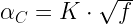 |
where
- K is constant that aggregates all the non-frequency dependent terms.
Equation 2 is of the form that will plot as a straight line on a log-log plot.
Graphical View of Coaxial Cable Attenuation
Figure 2 shows a log-log plot of Equation 1 and empirical data for an actual RG-6 cable (Belden 1694A) that is 100 feet long. You can see that the loss characteristic is tilted up.
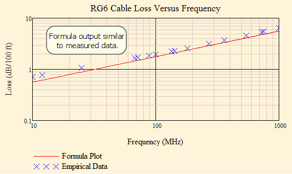
Figure 2: RG6 Loss (dB/100 ft) Versus Frequency.
Compensating for Frequency-Dependent Coaxial Cable Losses
From the standpoint of the television, the best way to ensure consistent picture quality is to make sure that every channel has the same voltage level at the television receiver. To ensure that every channel is received with the same signal level, our optical-to-RF converter (i.e. home receiver) would generate an output signal whose output voltage increases with increasing frequency just enough to cancel this increase in loss.
To perform this compensation, we need to make some assumptions.
- Our customers are using RG-6 coaxial cables.
This is the most common residential, coaxial cable used today. Occasionally, you do see some RG-59, but this is for short spans between a set-top box and a television.
- Our customers use 100 feet of coaxial cable in their homes.
The cable attenuation is rated in dB/meter, so longer cables have proportionately more loss. You have to assume some number for cable length and the industry has chosen to use 100 feet or 30 meters.
- Our customers will watch channels with a frequency range from 54 MHz to 1003 MHz.
This is the standard for the North American cable deployments. This is a very wide band and RG-6 has an attenuation range over this band from ~1 dB (54 MHz) to 6 dB (1003 MHz) per 100 feet of cable.
We design our video receivers to exactly compensate for the losses present on a 100 foot coaxial cable. This means that we output 17 dBmV at 54 MHz and linearly increase this voltage to 22 dBmV at 1003 MHz. The exact value of the voltage at the television set will depend on the value of the RF splitter that may be in the path. Televisions generally can reliably receive a signal in the range of 3 dBmV to 20 dBmV. It is a Goldilock's problem – less than 3 dBmV is not enough signal to reliably receive the signal and above 20 dBmV can cause receiver distortion.
Conclusion
Whether I have been designing sonar, radar, infrared, or television systems, I always have to deal with issues in the transmission medium. This post provides some background on how we compensate television signals for the frequency response of the coaxial cable.