Modeling Pulse Distortion
Choice of Pulse Basis Function
As with most modeling problems, it is very important to choose a function that accurately represents your physical signal. The most commonly used pulse models in optics are based on the normal curve. The normal curvea is described by the following equation.
where is the standard deviation and
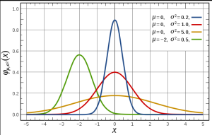
is the mean of the normal curve. The Wikipedia has a nice graph of the normal curve, which I include in Figure 2.
In this particular work, the pulse has its time (function f) and wavelength(function h) functions each modeled by different normal curves.
Eq 4.
where t is time, T is the fiber travel time for the center of the pulse, is the wavelength,
is the center wavelength of the pulse,
is the standard deviation of the pulse width in time, and
is the standard deviation of the pulse width in wavelength. For this discussion, we are going to ignore attenuation losses and focus on the effect of dispersion. It turns out that the losses due to attenuation are easy to add, but they add more bulk to this discussion that is already too long.
Modeling Pulse Dispersion Impact on Power
There are many textbooks that provide rigorous derivations of the equation we will be using to model pulse spreading. I will use a more intuitive argument here to motivate, but not prove, the use of this equation. We begin our discussion with a few observations.
- The pulse time function can be modeled as being composed of two normal signals: (1) the initial pulse shape, and (2) the standard deviation of the dispersed laser pulse.
- The variance of the sum of these two signals is the sum the variances.
- The standard deviation of the dispersed laser wavelengths is given by
.
These observations lead us to write down the following equation directly (a detailed proof involves convolutions).
Eq.5
where is the time-domain variance of the total waveform,
is time-domain variance of the initial pulse (t=0), L is the distance of pulse travel, and
is the standard deviation of the laser pulse.
Increasing will increase the pulse duration and reduce its amplitude, exactly what happens in a dispersed pulse. Substituting Eq. 5 into Eq. 4 gives us the equation of the dispersed pulse.
Eq. 6
A quick look at Equation 6 shows that its amplitude reduces with range by a factor of . This reduction in pulse amplitude means a reduction in power that can be modeled using Equation 7.
Eq. 7
All the commonly used dispersion power penalty formulas appear to be based on this equation. Given this equation, I now can demonstrate how Equations 1 through 4 (listed in part 1 of this blog series) were derived.
Equation Derivations
The only differences I can find between the equations are related to how one defines the relationship between the bit rate and . This relationship is set by the amount of ISI that the engineer can tolerate. Here is a quick summary of the assumptions behind each equation:
- Equation 1 assumes that the engineer wishes to define the bit time as equal to that of a rectangular pulse with the same energy and peak value as a normal pulse.
- Equation 2 assumes that the engineer wishes to define the bit time as the period required to contain 95% of the pulse energy at the time of transmission.
- Equation 3 assumes that the engineer wishes to define the bit time as the period required to contain 95% of the pulse energy at the time of reception.
- Equation 4 is Equation 3 with a Taylor series approximation applied.
With all this said, it is now time to dive into the details.
Deriving Equation 1
Equation 1 is derived from Equation 7 using the following assumptions.
- The pulse is specified to be of time duration T and amplitude P, which implies rectangular in shape.
- The Gaussian pulse equivalent has the same total energy and peak amplitude.
Given these assumptions and the fact that the area under a Gaussian pulse is , we can derive the
of the Gaussian pulse as follows.
Eq. 8
Given that the bit period T is related to bit rate B by , we can solve Eq. 8 for
to obtain Eq. 9.
Eq. 9
We can substitute Equation 9 into Equation 7 to obtain Equation 1.
The next blog will cover deriving Equations 2 – 4.


I just find your blog today, cause I got some task from school about dispersion power penalty. can you tell me some book or anything that I can use to complete my task. because my teacher don't suggest me to use a blog as a references. But until now only your blog that can help me, It's so hard to find any material about dispersion power penalty.
hanks a lot.
keep writing!
I will send you some papers that I used in my research. The only text I used was "Fiber Optic Communications Systems" by Agrawal.
Mathscinotes
You say that:
1) (x) is the standard deviation of the pulse width in wavelength
2) (x)^2 is the spectral width of the laser.
In (1) and (2), (x) is the same parameter? What is (x) ???
Sorry about the confusion -- my fault. The formulas assume that the laser’s spectrum can be modeled using a Gaussian shape. This shape is characterized by a standard deviation, which I called σλ. There is a relationship between spectral width and σλ, which I document here. I sometimes use spectral width and σλ interchangeably, however, they are different. They are related by a constant factor. I will update the blog post when I have time.
Mathscinotes