
Quote of the Day
If you complain, you make yourself a victim. Leave the situation, change the situation or accept it.
— Unknown
Introduction

Figure 1: Brake undergoing dynamometer tests. Brake pad failures are often modeled using a lognormal probability distribution. (Source)
I have spent some time lately talking to people about laser failure characteristics. Most electronic component reliability modeling is done using the exponential probability distribution, which assumes the components have a constant failure rate and there is no wear-out mechanism. It turns out that lasers have a wear-out mechanism, which means the exponential probability distribution is not appropriate. Laser failure rates are usually modeled by a lognormal probability distribution, as are the failure rates of brakes (Figure 1) and incandescent light bulbs. These components have reliabilities that are dominated by wear-out mechanisms that accelerate when damage to a small region grows exponentially. A good example would be a hard spot on a brake pad that becomes hot during braking relative to the rest of the pad. This hard spot tends grow quickly because the heat generated during braking concentrates there.
Lognormal Probability Distribution Basics
Equations 1 and 2 give the definitions of the lognormal probability density and cumulative probability distribution, respectively.
| Eq. 1 |  |
| Eq. 2 |  |
where μ is the mean and and σ is the standard deviation of the random iterate t.
The idea behind the distribution is simple – a random variable T is said to be lognormal distributed if log(T) is normally distributed. Figure 1 shows the shape of the lognormal density and distribution for μ = 1 and σ=1.
.")
Figure 1: Lognormal Example (Density and Cumulative Distribution) – μ = 1 and σ=1.
Empirical reliability studies have shown that the lognormal distribution provides a good model for components whose reliability is dominated by a wear-out mechanism.
Laser Reliability Physics
So why does nature demand the use of the lognormal distribution for wear-out problems? To motivate the use of the lognormal distribution, we need to understand how lasers fail. The laser puts out a specified amount of optical power (i.e. light) when driven with electrical current. As a laser ages, it takes more current to generate the required optical power. Eventually, the current required to obtain the required optical power exceeds the current limits of the electrical circuitry.
One way to model this behavior is to assume that there are one or more light-absorbing defects that are growing within the optical channel of the laser. This is a credible theory because these optical defects will be absorbing light, which provides the power needed for the defects to grow. To model this behavior, let a0, a1, …, an be a sequence of independent random variables representing the successive growth of the defect area. Let a0 be the initial defect area and an be the defect area that results in component failure. As the defect area increases, more optical power is absorbed and the rate of defect growth will increase. Equation 3 can be used to model this characteristic.
| Eq. 3 |  |
This means that we can express an as a product in terms of a0 and the δi's as shown in Equation 4.
| Eq. 4 |  |
If we take the logarithm of both sides of Equation 3 and assume that the δi's are much less than 1 , we obtain Equation 5.
| Eq. 5 |  |
We can use the central limit theorem and the assumption that that the δi's are independently distributed random variables to state that Equation 5 will converge to a normal distribution. Since the logarithm of the random variable an has a normal distribution, we see that an has a lognormal distribution.
A Real-Life Laser Reliability Example
Typical Laser Reliability Parameter Example
I will walk through an actual laser reliability specification and show where all the terms come from. I have used the laser with the reliability characteristics shown in Table 1. Note that wear-out specifications from laser vendors assume the laser is on all the time. For many systems, like PONs, the laser is only on a fraction of the time.

Table 1: Example of Typical Laser Reliability Parameters.
The key data in this table are the following items:
- σ
- Ea
- median life estimate at one temperature
Given this data, the rest of the information in the table can be computed, as I will show below. These key pieces of data are determined in an accelerated life study. This study takes a large number of lasers and stresses them under temperature to simulate operation over a long time interval. The key assumption here is that component aging is modeled by Equation 6, the Arrhenius equation.
Arrhenius Equation
Because it takes many years to get lasers at normal temperature to fail, we use temperature to accelerate the aging process for lasers. The aging of lasers is governed by the Arrhenius equation (Equation 6).
| Eq. 6 | 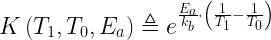 |
where T1 is the temperature at which we desire the failure rate, T0 is the reference temperature, and Ea is the activation energy.
The Arrhenius equation is used to estimate the failure rate at relatively low temperatures based on the test results from a large numbers of parts operating at high temperature. In Table 2, I have included some commonly seen activation energies for different failure modes.
| Mechanism | Activation Energy (eV) |
| Gross Coarsening in Solder | 0.42 |
| Intermetallic Defect | 0.3 |
| Metallization Defect | 0.5 |
| Line Electromigration | 0.45 – 1.2 |
| Dark Line Defects in AlGaAs/GaAs Lasers | 0.2 |
| Gradual Degradation in AlGaAs/GaAs LEDs | 0.5 |
For the laser used in my example here, the activation energy is 0.4 eV. This number is always listed by the laser vendor and it varies a bit depending on the characteristics of their processes.
Definition of Failure Rate
There are a number of terms that are often erroneously used interchangeably to describe failure rates.
- failure rate
- instantaneous failure rate
- hazard rate
Each of these terms actually has a distinct meaning. This paper will use the term hazard rate, which is the standard method for lasers.
The hazard rate, h(t), is actually a conditional failure rate defined in Equation 7.
| Eq. 7 |  |
The term 1-F(t, µ, σ) is sometimes referred to as the survival function.
Mathcad Calculations
I grabbed all the equations from the Wikipedia. Figure 2 shows the equations as implemented in Mathcad. Note that Mathcad has built-in functions for the lognormal density and cumulative distributions. I chose not to use them just to illustrate how these functions could be implemented in other tools.

Figure 2: Mathcad Implementation of Equations.
Figure 3 shows how to calculate all the terms in Table 1.

Figure 3: Reproduction of the Laser Reliabilty Results in Table 1.
Conclusion
I was able to demonstrate how laser reliability results are calculated. Hopefully, this post will remove some of the mystery behind how laser reliability numbers are computed.
I would like to understand the failure mechanism of a laser diode operating i high temperature. What for instance is the main failure mechanism of 40mW 1550nm laser diode operating at 85 deg C, at 120 deg C? I understand current and optical power both have an effect. What if the laser is not operating and just subjected to high ambient temperature?
My focus in this post was laser wearout. Like all electronic components, lasers are subject to corrosion and contamination problems that are exponentially driven by temperature. These failure mechanisms are driven by a part's time at temperature and not its operating time. Many laser reliability specifications have a random wearout term to reflect this failure mode. This term gives a constant failure rate that describes an exponential (memory-less) probability characteristic. This same characteristic is used for nearly all electronic parts because these parts generally have a constant failure rate.
Pingback: Thermal Calculation Example for a Simple Electronic Component | Math Encounters Blog