Dimensional Analysis and Olympic Rowing

Introduction

I have always found dimensional analysis to be a very useful engineering tool. I recently watched a video Professor John Barrow of Gresham College who did a very nice job illustrating how dimensional analysis can be used to derive useful results. One example that particularly intrigued me involved Olympic rowing. Using dimensional analysis, he was able to derive a relationship between the crew size of a rowboat and its speed. He then curve fit the results from the 1980 Olympics to his relationship and showed that for one Olympic year there was good agreement. I thought it would be a good illustration of the power of Mathcad's curve fitting routines to show how easy it is to extend this analysis to multiple Olympic years.

Background

I am not a rower, but I will summarize the small amount that I needed to know to model rowboat velocity versus the number of rowers.

• Coxless Versus Coxed
  The crews of rowboats consists of rowers and an optional coxswain (often shortened to cox). The cox will steer and keep the pace.
• Course Length
  Races are over a 2000 meter course.
• Crew sizes
  For this exercise, I will be looking at coxless gold medal scores with 1, 2, or 4 male rowers. I will also examine coxed gold medal scores for 2,4, and 8 male rower crews.
• Speed Calculation
  I will be looking at over speed, v, over the course, which I compute using .

Analysis

While I recommend Professor Barrow's lecture for the details of showing that rowboat velocity increases with the 9th root of the number of rower, I do summarize his derivation in Equation 1. It is terse, but you can get the gist of the argument.

Eq. 1
	By Archimedes law, displaced volume increases linearly with the number of rowers. This means the wetted area increases by the 2/3 power of the number of rowers.

A similar derivation is shown in Equation 2 for a coxed rowboat, assuming the cox weights half that of a rower.

Eq. 2

Coxless Rowing (Equation 1)

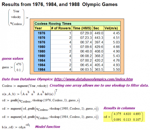
I will now use Mathcad to fit Olympic rowing data to the 9th root curve. Figure 1 summarizes my results for the Olympic gold medal results of 1976, 1980, and 1984 for coxless 1, 2, and 4 man rowboats.

Figure 1: Coxless Rowing Analysis Results.

Coxed Rowing (Equation 2)

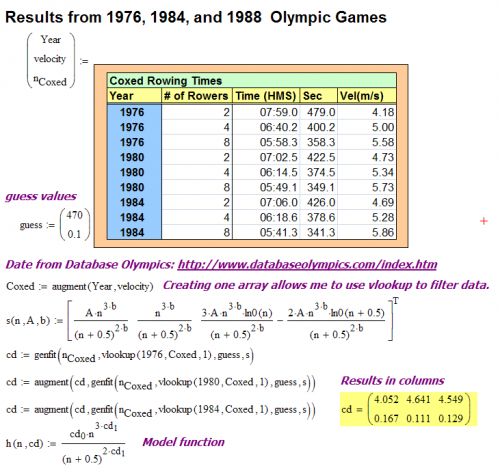
The difference between Equations 1 and 2 is that cox adds weight and no power. I will now use Mathcad to fit Olympic rowing data to Equation 2. Figure 1 summarizes my results for the Olympic gold medal results of 1976, 1980, and 1984 for coxed 2, 4, and 8 man rowboats.

Figure 2: Coxed Rowing Analysis Results.

Conclusion

Considering the crudeness of the model, the results were not too bad. It was a nice use of dimensional analysis to gain insight into a problem. The main issue I have with the model lies in the estimate of the wetted surface area. But Professor Barrow's approach is a great first-order approximation. If I was looking for improvements, I might look closer at that wetted surface area equation.