
Introduction

Figure 1: HDTV is now the norm.
Everyday, I work on delivering fiber-based, video access equipment to service providers. The increased demand for High-Definition Television (HDTV, Figure 1) has increased the need for fiber in the video distribution network. Today, fiber optic cable is often used to deliver the video signal to "green yard furniture" (Figure 2) in local neighborhoods that convert the light to electrical form for distribution using copper-based technologies, like cable TV or DSL.

Figure 2: Green Yard Furniture (Source).
Increasingly often, optical fiber is being used to deliver the video directly to the home – this is the focus of my work. As part of preparing some tutorial material on video distribution, I needed to explain how these distribution networks are configured. There was some interesting math involved in this work that I thought would be interesting to share here.
Background
Objective
In this post, I will look at how optical video transmission performance is determined by two key parameters, composite RMS OMI and channel peak OMI (defined below). These parameters are difficult for customers to understand, but critical to the performance of their networks.
A relationship will be determined between these two parameters that is used every day in my lab to setup video systems. This analysis will uses some basic probability theory and calculus to derive a useful result.
Multi-Channel Video Transmission Basics
There are two basic types of video transmission:
- IP-based
The video data is shipped in digital form like any other internet data. This is being rolled out now and is the future of television. IP-based video subscribers receive only the channels that they are watching. This service is only now being deployed and it will take years before everyone gets access to it.
- RF-based
RF-based video broadcasts multiple channels on the fiber in a manner similar to how over-the-air channels are broadcast – every channel gets a frequency assignment in the band from 54 MHz to 1003 MHz. Each video channel is encoded in an analog form (e.g. NTSC or QAM), summed together, and that sum used to modulated a laser. The video signal itself is carried on a separate wavelength, usually 1550 nm.
This post will focus on the RF-based approach. This approach is becoming less common, but there are still tens of millions of people who watch TV using this technology.
I have been told every year over the last 15 years that RF-based video is going to die in the next two years. I expect to retire in ten years with tens of millions of people still watching RF-based video. Change comes slowly in the access network.
Figure 3 shows the basic video distribution network.

Figure 3: RF-Based Video Model.
In Figure 3, a large number of electrical channels go into the laser and the same number of electrical channels come out of each home's optical receiver. In this respect, it is similar to how an over-the-air broadcast works.
Definitions
Aspects of these definitions may require some additional background for those unfamiliar with amplitude-modulated system. See Appendix A for some additional background on these systems.
- Carrier-to-Noise Ratio (CNR)
- CNR is the carrier power-to-noise power ratio and it is the primary quality metric used with respect to analog video. For the purposes of this article, you should think of CNR and SNR as being synonymous – technically they are different, but are close enough that we will not draw a fine distinction. If you want more details on the difference, see this note. The higher a channel's CNR, the better the video quality.
- Clipping-Induced Distortion
- Video distribution works by electrically summing a large number of channels (~100) and feeding this sum into the front-end of a laser. The laser generates optical power that is directly proportional to its electrical input. However, optical power can never be negative in value, but an electrical signal can be negative. To avoid this issue, the laser is "biased" to generate a constant output power level with zero electrical input. In this way, we can use a non-negative parameter like power to represent a signed value like electrical voltage. However, it turns out that the electrical signal can randomly have negative values so large that its the sum of electrical signal can be negative and the laser generates zero output power when the input is negative. Figure 4 illustrates this situation.
-

Figure 4: Illustration of Clipping.
In theory, you could make the laser bias large enough to ensure that the input cannot be negative. However, there are limits to the amount of power you can transmit down a fiber because of nonlinearities like SBS. Also, higher laser power means MUCH higher cost.
The loss of signal, while short, creates a distortion in the television signal. We refer to this distortion as clipping-induced distortion.
- Channel Peak OMI (symbol m)
- m represents the ratio of maximum optical power deviation (one-sided) for a single channel to that channel's total optical power. The larger m, the higher the CNR of that channel. We can describe it mathematically as follows.
Most cable systems support two OMI levels: one for analog channels and one for digital channels. QAM256 is the most common type of digital channel and it is usually set at 50% of the analog level.
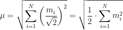
- Composite RMS OMI (symbol µ)
- Composite RMS OMI is defined as the RMS optical power deviation (one-sided) to the total optical power for a multi-channel system. We can describe it mathematically as follows.
The amount of clipping-induced distortion is related to the composite RMS OMI. The number of channels that can be transmitted on a single wavelength is a function of the channel peak OMI, the number of channels, and allowed composite RMS OMI for a given level of clipping induced distortion. I will be investigating this relationship closely.
The factor of two appears because the channel peak OMI must be converted to an RMS value for the composite calculation. If all the OMI values are the same (e.g. an all analog system), then
.


Analysis
Clipped Power
Equation 1 shows formula for the amount of power that was present in the electrical signal but is clipped from the optical signal. You will note that the integral involves the optical power squared and not just the power. This has to do with a subtlety of optical systems in that a milliWatt of optical power produces so many milliAmps of electrical current in the receiver. This means that the electrical signal power produced by the receiver, which is related to the square of electrical current, is proportional the square of the optical power. To compute the electrical power that was clipped, we need to compute the integral of the optical power squared times the probability of clipping, which is Equation 1.
| Eq. 1 | 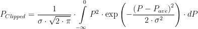 |
where
- P is the optical composite power (all channels together) on the fiber.
- Pave is the average optical composite power on the fiber, which is also referred to as the bias value.
- σ is the standard deviation of the optical composite power signal on the fiber.
For this analysis, I am going to assume that the system performance is limited by clipping-induced distortion. Figure 5 shows my derivation for the power that was clipped from the original signal (highlighted in yellow).

Figure 5: Clipped Power Signal Derivation.
Carrier-to-Clipping Power Versus Composite OMI
Figure 6 shows how to derive the Carrier-to-Clipped Power of the composite system as a function of the composite OMI. Note that σ represents the standard deviation of the optical power and σ2 represents the electrical power of the information content of the video signal, which is called the signal power.

Figure 6: Derivation of Carrier-to-Clipped Power.
The equation highlighted in yellow is well-known in the industry as the Saleh equation (ref: A. A. M. Saleh. Fundamental limit on number of channels in subcarrier-multiplexed lightwave CATV system. Electron. Letters, 25(12):776-777, 1989). You will sometimes see this equation in a slightly different form (see Appendix B).
Example System Configuration
Clipping-induced distortion is only one of a number of noise source in a video system (e.g. RIN, thermal, shot), but it is often a dominant one. Figure 7 shows an example of OMI calculations for a commonly used system configuration consisting of:
- 80 analog channels, which require a minimum of 3.8% peak channel OMI to meet minimum quality standards (CNR>48 dB).
There is some debate on the actual CNR requirements. The FCC minimum CNR is 43 dB, which produces a picture with quality comparable to that of an old VHS tape player. A few service providers use 46 dB, but most use 48 dB.
- 33 digital channels, which require a minimum of 1.9% peak channel OMI to meet minimum quality standards (Modulation Error Ratio [MER]>35 dB).
As mentioned earlier, this level is typically set at half of the analog level for QAM256, i.e. 1.9% = 3.8%/2.
- clipping induced distortion 58 dB less than the carrier.
We typically set clipping induced distortion to a level at 10 dB less than the required CNR level of 48 dB.
The calculation shows that we just meet our minimum requirements with 80 analog and 33 digital channels.
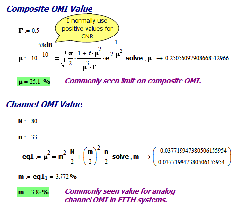
Figure 7: Worked Example for Composite and Channel OMIs for Common Layout.
Conclusion
I frequently am asked why RF-based video has to be setup a certain way or it just does not work well. Hopefully, these calculations show where some of the odd ball formulas come from and that deriving them is not simple.
Appendix A: AM-VSB Channel Model
We generally test the AM-VSB channels using a unmodulated carriers. We can model the optical power present in this test configuration as shown in Equation 2.
| Eq. 2 |  |
where
- P0 is the average optical power level.
- mi is the OMI of the mth channel.
- fi is frequency of the ith channel.
- N is the total number of channels.
- pOptical is the instantaneous optical power.
- xi is the ith channel signal level normalized to P0. which means that x(t) represents the ith channel level with an mean value of 1.
Equation 2 can be thought of as using optical power to represent the voltage of the original television signal, i.e. 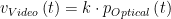
The optical receiver contains a photodetector that generates a current proportional to the input optical power. This means that we can express the detector's output current as shown in Equation 3.
| Eq. 3 |  |
where
- Z0 is the characteristic impedance of the system (75Ω in video systems)
- R is the responsivity of the photodetector [A/W].
- vReceived(t)is the RF voltage generated by the receiver output current being driven into Z0. vReceived(t) is a scaled representation of the original signal vVideo(t).
In general, there are on the order of 80 analog video channels multiplexed on a single laser output. We can think of vReceived(t) as the sum of a large number (~80) independent, identically distributed, random variables. Because of the central limit theorem, vReceived(t) is well-modeled as a Gaussian random process with mean R·P0 and variance of 
We define the composite modulation index (µ) as the standard deviation (σ) normalized to the signal mean of vReceived(t), R·P0, which I show in Equation 4.
| Eq. 4 |  |
Appendix B: Another Form of Saleh Equation
Some folks like to express CNR as a negative dB value and with a numeric constant for a leading coefficient (example). Figure 7 shows how to derive this expression.

Figure 7: Alternative Form of Saleh Equation.