
Quote of the Day
Every politician's goal is to get the credit for something popular that would have happened anyway.
— Philip Bump, political commentator
Introduction

Figure 1: Pejsa's F Function Reference.
I have had several people ask me to review how Pejsa generated his F function. Recall that Pejsa's approach is based on using a parameter called the ballistic coefficient (BC) to scale the performance of a reference projectile – Pejsa used the US military's 30 caliber M2 bullet, which dates back to the Springfield rifle. This effort involves basic curve fitting, and I will illustrate the process for the velocity interval from 1400 feet per second (fps) to 4000 fps. This velocity range is the most important to most folks and it illustrates the basic curve fitting process well.
Pejsa actually defined four velocity intervals (Pejsa numbered them in this order):
- 0 fps to 900 fps
- 900 fps to 1200 fps
- 1200 fps to 1400 fps
- 1400 fps to 4000 fps
As can be seen in Figure 1, two of the velocity intervals (#2 and #4) are simple horizontal lines and no fitting activity is needed. I will leave fitting velocity interval #3 to others, but the process is the same as shown for fitting velocity interval #1 below.
Background
Projectile Types
Some of the questions I have received indicate that it is not clear to people that there are many reference projectile shapes. Figure 2 shows the drag coefficients (related to the 1/F function) for a few of the common reference projectiles. Of all of these, G1 is by far the most common, but G7 is growing in popularity.
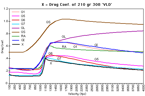
Figure 2: There are Numerous Reference Projectiles.
Pejsa's approach was to create his own reference projectile based on the M2 and scaled his results in a manner that would allow the use of G1 BCs, which are commonly available.
You do not see the Pejsa reference projectile mentioned much because Pejsa never explicitly presented it. However, you do occasionally see it (Figure 3 calls it "GP") presented on some web pages.

Figure 3: Set of Drag Coefficients for Reference Projectiles, Including Pejsa's (source).
In Appendix A, I explain how to generate the reference projectile curve from Pejsa's model.
Analysis
Data Capture
Figure 4 shows the data that I captured from Figure 1 using Dagra.

Figure 4: Data Captured from the Upper Curve of Figure 1.
Curve Fitting
Figure 5 shows the curve fitting process that I used for data captured from Figure 1.

Figure 5: Curve Fitting the Data from Figure 1.
Equation 1 shows the result of my curve fitting.
| Eq. 1 | 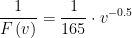 |
where
- v is the projectile's velocity [fps]
- F(v) is Pejsa's F function [ft]
The only difference between my result and Pejsa is that his coefficient is 166 and mine is 165. This is excellent agreement considering I am working off of a poor quality image.
Quality of Curve Fit
Figure 6 shows the quality of my curve fit to the data I captured.

Figure 6: Curve Fit Quality.
While I have confirmed my fit equation closely models my data, I still need to show how closely my curve matches Pejsa's. Figure 7 shows that my curve is within 2.5% of Pejsa's result along the entire curve.

Figure 7: Cross Checking My Result with Pejsa's.
Conclusion
This post shows how you can generate Pejsa's F function for yourself based on the 30 caliber M2 drag data. This same approach could be used to extend Pejsa's approach to other reference projectiles – a task that I will leave to others.
Appendix A: Drag Coefficient vs Pejsa's 1/F Function
Most work on projectiles is done using drag functions. Pejsa's 1/F function is closely related to standard drag functions – a relationship that I demonstrate in Figure 8.
An equivalent drag function can be derived from Pejsa 1/F function for a 30 caliber M2 bullet (Figure 1). Note that this is not the 1/F function for a reference round (1 inch diameter, 1 pound mass). You can generate the reference 1/F by dividing the 1/F function of the M2 bullet by its ballistic coefficient, which is 0.484. This is exactly what Pejsa did.
Pejsa does briefly mention drag functions, but then omits a factor of 1/2 in his formulation. In modern work, we normally see a factor of 1/2 in the drag formula and I included it in my work below. This factor of 1/2 is needed to obtain the same results for the Pejsa reference projectile that others obtain.

Figure 8: Demonstration of Equivalence Between 1/F and Drag Function.
Pingback: Drag Coefficient From A Ballistic Drop Table | Math Encounters Blog
I just ran into your blog while researching on ballistics, trajectory and drag. Very nicely done body of work. I noticed in your July 1, 2015 posting the equation 1 curve fitting result and looking at the the graph figure 6 that they disagree by what looks like a factor of 2. Right side is graphed as 2/165 * v^(-.5). Is that correct? I thought I read somewhere on one of your postings that Pejsa halved his F function?
I have really enjoyed your ballistic blogs but I'm still no closer to being able to generate the G1 table of standard drag coefficients. However much I've trawled the internet I can't find the elusive equation to calculate Drag Force or Drag Coefficient without having either value.
You mentioned Wikipedia as a good reference on the Drag Equation and Drag Coefficient. I think, given your particular set of skills, you should run your eye over their content on the Ballistic Coefficient. I think there may be some shortcomings in their equations for the calculation of i, n and Cd. They say Cd can be calculated mathematically but the equation they use includes p = projectile density where I suspect they mean Air Density and pi().d^2 where I suspect they may mean the cross-sectional area being pi().(d/2)^2. In any case, I haven't been able to make use of this equation to calculate Cd.
I'm clearly missing something very obvious and admit that algebra is not one of my strengths.
Thank you once again for your blogs.