Quote of the Day
Truth … is much too complicated to allow anything but approximation.
— John von Neumann. It took me a long time to accept that all models are wrong at some level, but that you can use them to produce useful results.
Introduction

Figure 1: Observatories are usually placed on
remote mountaintops. Here is a picture of the
Sphinx Observatory (Source).
I often see popular descriptions of observatories that say things like the observatory "is above 40% of the Earth's atmosphere". I had not thought much about this kind of statement until I saw the Wikipedia's list of the world's highest-altitude observatories, which surprised me as to the height and remoteness of the largest telescopes. I cannot imagine trying to build on these locations (Figure 1 is an extreme example). In some respects, the construction challenges remind me of what builders must have gone through on some lighthouses.
In this post, I will look at the highest altitude observatories and compute the percentage of atmosphere that they are above.
Background
The atmospheric pressure at a location is a measure of the weight of air above that location. We can determine the percentage of the air column below a given altitude by computing the ratio of p(h)/p(0), which represents the percentage of atmosphere above altitude h , and subtracting that ratio from 100%.
| Eq. 1 | 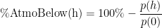 |
where
- %AtmoBelow(h) is the percentage of atmosphere below the altitude h.
- p(h) is the atmospheric pressure at altitude h.
- p(0) is the atmospheric pressure at sea level, h= 0.
In this post, I will:
- Verify some general statements about the amount of atmosphere below certain altitudes.
- Determine the amount of atmosphere below the world's highest observatories.
Analysis
Atmospheric Pressure Curve Fit
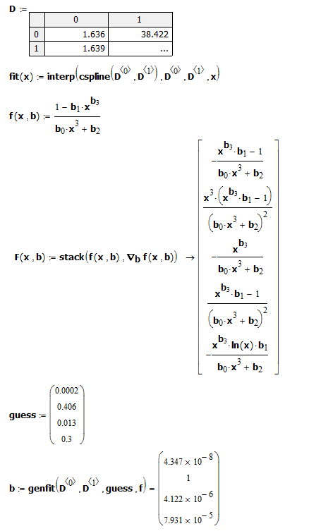
To estimate the barometric pressure at different altitudes, I grabbed a table of pressures from the web and did a simple interpolation so that my function, p(h), is continuous (Figure 2).

Figure 2: Mathcad Interpolation of Barometric Pressure.
Web References
Table 1 shows three examples of references to the percentage of atmosphere below that reference level. Note that the reference for Everest (marked in red) got their percentage number wrong by ~10%.
| Statement | Altitude (m) | Stated Air % Below | My Air % Below |
| Mauna Kea rises 9,750 meters from the ocean floor to an altitude of 4,205 meters above sea level, which places its summit above 40 percent of the Earth's atmosphere (Source). | 4,205 | 40 | 40.8% |
| 57.8 percent of the atmosphere is below the summit of Mount Everest (Source). | 8,848 | 57.8 | 68.9 |
| 72 percent of the atmosphere is below the common cruising altitude of commercial airliners (about 10,000 m) (Source). | 10,000 | 72 | 73.8 |
Figure 3 shows how the calculation was performed using Equation 1.

Figure 3: Example Calculations.
World's Highest Observatories
The Wikipedia has a list of the highest observatories in the world. I used Equation 1 to find the percentage of atmosphere below each observatory in Table 2. The University of Tokyo Atacama Observatory is unbelievably high – that has to be a challenge for those who work there.
| Observatory Name | Elev.(m) |
Air % Below | Observatory Site | Location |
| University of Tokyo Atacama Observatory (TAO) | 5,640 | 51.0% | Cerro Chajnantor | Atacama Desert, Chile |
| Chacaltaya Astrophysical Observatory | 5,230 | 48.3% | Chacaltaya | Andes, Bolivia |
| James Ax Observatory | 5,200 | 48.0% | Cerro Toco | Atacama Desert, Chile |
| Atacama Cosmology Telescope | 5,190 | 48.0% | Cerro Toco | Atacama Desert, Chile |
| Llano de Chajnantor Observatory | 5,104 | 47.4% | Llano de Chajnantor | Atacama Desert, Chile |
| Shiquanhe Observatory (NAOC Ali Observatory) |
5,100 | 47.4% | Shiquanhe, Ngari Plateau | Tibet Autonomous Region, China |
| Llano de Chajnantor Observatory | 4,800 | 45.2% | Pampa La Bola | Atacama Desert, Chile |
| Large Millimeter Telescope Alfonso Serrano | 4,580 | 43.6% | Sierra Negra | Puebla, Mexico |
| Indian Astronomical Observatory | 4,500 | 43.0% | Hanle | Ladakh, India |
| Meyer-Womble Observatory | 4,312 | 41.6% | Mount Evans | Colorado, United States |
| Yangbajing International Cosmic Ray Observatory | 4,300 | 41.5% | Yangbajain | Tibet Autonomous Region, China |
| Mauna Kea Observatory | 4,190 | 40.7% | Mauna Kea | Hawaii, United States |
| High-Altitude Water Cherenkov (HAWC) Gamma-Ray Observatory | 4,100 | 40.0% | Sierra Negra | Puebla, Mexico |
| Barcroft Observatory | 3,890 | 38.3% | White Mountain Peak | California, United States |
| Very Long Baseline Array (VLBA), Mauna Kea Site | 3,730 | 37.0% | Mauna Kea | Hawaii, United States |
| Llano del Hato National Astronomical Observatory | 3,600 | 36.0% | Llano del Hato | Andes, Venezuela |
| Sphinx Observatory | 3,571 | 35.7% | Jungfraujoch | Bernese Alps, Switzerland |
| Mauna Loa Observatory | 3,394 | 34.3% | Mauna Loa | Hawaii, United States |
| Magdalena Ridge Observatory | 3,230 | 32.8% | South Baldy | New Mexico, United States |
| Mount Graham International Observatory | 3,191 | 32.5% | Mount Graham | Arizona, United States |
| Gornergrat Observatory | 3,135 | 32.0% | Gornergrat | Pennine Alps, Switzerland |
| European Extremely Large Telescope | 3,060 | 31.4% | Cerro Armazones | Atacama Desert, Chile |
| Haleakala Observatory | 3,036 | 31.2% | Haleakala | Hawaii, United States |
Conclusion
Just a quick note to explain where some of these atmosphere percentage numbers come from. I became interested in this after watching the movie Everest, which did an excellent job showing the effect of high altitudes on people.