When I was a child (late 1950s and early 1960s), there were many discussions of about a rotating space "wheel" – Wernher von Braun was a key proponent for developing this type of space station (Figure 2). There was even a horrible feature film made about the subject, Conquest of Space – a truly awful plot with pretty good special effects.
Figure 2: Rotating Space Wheel Proposal.
I found the new discussions interesting because they are discussing rotation rates and the fraction of Earth's gravity they wish to achieve. NASA even has a project called Nautilus-X that they want to use to determine the requirements for an artificial gravity system.
In this post, I will derive a pair of expressions for determining:
rotation rate as a function of desired artificial gravity level (i.e. percentage of the Earth's gravity).
artificial gravity level as a function of space station radius and rotation rate.
Background
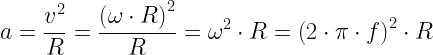
All of these space station proposals generate artificial gravity using centrifugal force. Equation 1 gives the centrifugal acceleration as a function of velocity and radius. This formula forms the basis of my mathematical argument.
Eq. 1
where
ω is the angular velocity of the space station [radians/sec].
f is the revolutions per minute of the space station.
v is the tangential velocity of a person on the space station rim.
R is the radius of the space station.
Analysis
Scope
I will look at the space station characteristics from three proposals:
Original von Braun proposal.
United Space Structures proposal
Nautilus-X table of diameters and rates
Derivations
Figure 3 shows how I derived the formulas I needed using Mathcad.
Figure 3: Derivation of the Rotation Rate and Artificial Gravity Formulas.
Example Calculations
Figure 4 shows my calculations for the three examples mentioned above.
Figure 4: Calculation for 3 Examples.
I was able to duplicate all of their calculated values to a reasonable level of accuracy.
Conclusion
I have seen this discussion occur before – I hope this time someone actually builds a rotating space station. It is hard to believe, but after all these years we really do not have human data on the effects of generating artificial gravity using centrifugal force. There was one case where micro-gravity was generated during Gemini 11 in 1966 (Gemini spacecraft tethered to Agena target vehicle) and there is a proposal to use a tethered booster-Soyuz combination to run an artificial gravity experiment as part of an International Space Station resupply mission.
Posted inAstronomy|Comments Off on Space Station Math
The scientist is interested in the right answer, the engineer in the best answer now.
Introduction
Figure 1: Natural Nuclear Reactor at Oklo Exposed By Mining Operations. For scale purposes, I have red circled a person.
I read an interesting article today about the natural nuclear reactors of Oklo, Gabon. I had first read about these reactors in a Scientific American article back in 2005. The article I read today was interesting because it did a good job presenting some of the key numbers related to uranium isotope ratios on Earth, how the uranium got here, and how natural nuclear reactors could have formed ~2 billion years ago, but probably not today.
To help me understand the isotope ratios presented in this article, this post will develop an expression for how the isotope ratio of 235U to 238U has varied over time and this expression will be used to explain how conditions in Oklo two billion years ago were just right to form a natural nuclear reactor. In addition, I will use this model to estimate when the uranium was formed in a supernova explosion prior to the formation of our solar system.
Background
History
French researchers discovered the reactors in 1972 while performing an isotope analysis on rock samples from the Oklo site. The 235U-to-238U isotope ratio is normally very close to 0.72%, but at Oklo the ratio is 0.717%. While this may seem like a small deviation, the natural isotope ratio normally has little variance and the Oklo measurement were significantly outside the normal range. Detailed measurements of isotope residues conclusively showed that Oklo's 235U-to-238U isotope ratio was low because a nuclear reaction had consumed some 235U.
Video Briefing
Figure 2 shows a video briefing on the Oklo reactors that provides useful background information.
Figure 2: Video Briefing on Oklo Natural Reactors.
Geology
Figure 3(a) shows the location of the Oklo reactors on the African continent. Figure 3(b) shows the appearance of one of the reactors when a tunnel was dug through it.
Figure 3(a): Location of Gabon's Natural Nuclear Reactors (Link)
Figure 3(b): Appearance of the Underground Strata at Oklo.
Figure 4 is an illustration that shows how the natural reactors are positioned in the strata.
The following Wikipedia quote gives a good description of the number of reactors and their power level.
Oklo is the only known location for this in the world and consists of 16 sites at which self-sustaining nuclear fission reactions took place approximately 1.7 billion years ago, and ran for a few hundred thousand years, averaging 100 kW of thermal power during that time.
Reactor Operation
The following excerpt from the Wikipedia describes how the reactors would turn off and on periodically.
The natural nuclear reactor formed when a uranium-rich mineral deposit became inundated with groundwater that acted as a neutron moderator, and a nuclear chain reaction took place. The heat generated from the nuclear fission caused the groundwater to boil away, which slowed or stopped the reaction. After cooling of the mineral deposit, the water returned and the reaction started again. These fission reactions were sustained for hundreds of thousands of years, until a chain reaction could no longer be supported.
.... The concentrations of xenon isotopes, found trapped in mineral formations 2 billion years later, make it possible to calculate the specific time intervals of reactor operation: approximately 30 minutes of criticality followed by 2 hours and 30 minutes of cooling down to complete a 3-hour cycle.
Analysis
Stated Isotope Ratios
The article that I read presented the following numbers:
Uranium Isotope Ratio when the Solar System Was Formed
The article stated that the 235U to 238U ratio at the time of the solar system formation was ~17%. Here is the quote:
The most useful uranium isotope for nuclear power is uranium-235, which today accounts for just 0.7202% of any given natural sample of uranium. When the solar system first formed, that number would have been more like 17%, falling steadily until it reached the modern day value.
Uranium Isotope Ratio when Oklo Reactor was Operating
The article stated that the 235U to 238U ratio at the time the Oklo reactors were active was 3.6%, which was about 2 billion years ago. Here is the quote.
And 2 billion years ago? Scientists estimate the Oklo reactors would have had samples with roughly 3.6% uranium-235 — that’s close to the enrichment threshold of modern nuclear reactors. However, just packing the right material into a closed space does not a power plant make.
Today's 235U to 238U ratio of 0.72% is much lower than the 3.6% of 2 billion years ago and creating a natural nuclear reactor would be very difficult. You can create a nuclear reactor using natural uranium, but it is not easy (example). However, there is a fringe theory in geophysics today about a natural nuclear reactor at the Earth's core.
All the uranium isotopes in our solar system were created during a supernova explosion that occurred long before the Earth came into being.
The 235U to 238U ratio after a supernova explosion is 1.65 to 1 (source).
The article states that the 235U to 238U ratio was 17% "when the solar system formed". For this post, "when the solar system formed" means 4 billion years ago, which was the time the late heavy planetesimal bombardment stopped (source).
Given these assumptions, we can now perform the calculations shown in Figure 5. As part of my isotope ratio calculations, I also estimated that the supernova that created our solar system must have occurred ~6.5 billion years ago, which agrees with the value given by this source.
Figure 5: Isotope Ratio Calculations.
Conclusion
I was able to duplicate the article's results for the 235U to 238U isotope ratios of:
17% for the early Earth.
3.6% for the time when the Oklo reactor was active.
As a bonus, I was able to use the same model to compute that a supernova occurred 6.5 billion years ago that produced the material for our solar system.
All Plutophiles are based in America. If you go to other countries, they have much less of an attachment to either the existence or preservation of Pluto as a planet.
Figure 1: Pluto and its Moons As Seen from Earth. The Earth-Moon System diameter is about 770,000 km.
I have been following the voyage of the New Horizons spacecraft to Pluto (Figure 1) since its launch on January 19, 2006. It will flyby Pluto on July 14, 2015. I have already marked that day on my calendar!
I was reading the Planetary Society's blog post called "The Mapping of Pluto Begins Today" and the post mentioned that the Pluto is now large enough to form an image 3.5 pixels in width and height in New Horizons' narrow-field telescope. I thought it would be interesting to show how this calculation is performed.
To calculate Pluto's pixel width in New Horizon's telescope (Submarine Fiber-Optic Cable Trivia), you need to know the following numbers:
My calculation for Pluto's pixel width is shown in Figure 2, which confirms the 3.5 pixel width statement mentioned in the Planetary Society's blog post.
Figure 2: Calculations for the Pixel Width of Pluto in New Horizon's Narrow-Field Telescope on 20-March-2015.
I am not on my usual computer, so I did not have Mathcad available. I used Smath instead, which proved to be a workable substitute for this problem.
Posted inAstronomy|Comments Off on New Horizons Spacecraft Nearing Pluto
Hell, there are no rules here - we're trying to accomplish something.
Introduction
Figure 1: Fiber-Optic Cable Being Hooked Up To A Shore Facility. (Source)
I am at the Optical Fiber Conference in Los Angeles this week and learning a lot. For example, this morning I attended a great talk submarine fiber optic cables given by Neal Bergano, CTO of TE Connectivity Subcom. I thought I would put my mental notes on a post for others to view. I was not able to find a copy of Neal's presentation, so I just recalled what I could. Where possible, I will include supporting information that I located on the web. Any errors introduced are mine.
If you are interested, I have discussed these cables in other posts (here and here), but not at this level of detail.
Fun Submarine Fiber-Optic Cable Facts
All the continents but Antarctica are connected by fiber optic cables.
Figure 2 shows how extensive the world's network of submarine fiber optic cables has become (source).
Figure 2: World Fiber Optic Deployments.
99% of the world's transoceanic traffic goes over submarine cables.
He said that no one knows what the real number is. It could be 99.999%, but people hedge their bets by saying 99%.
Submarine Fiber-Optic Cables Include Power Amplifiers, Gain Equalizers, and Branching Units.
Submarine cable systems include more than just fiber. They also include the following "bumps" in the cable:
Repeaters (Erbium-Doped Fiber Amplifier [EDFA]) to restore signals levels lost because of attenuation over distance.
My web research shows the repeaters are placed every 60 km or so.
Gain Equalizers to ensure all wavelengths (i.e. colors) are maintained at the same level on the fiber.
Each wavelength experiences different losses on the fiber. The equalizer will introduce different levels of amplification for each wavelength to make their power levels equal.
Branching Units for connecting sites far from the main fiber ring.
If you look carefully at Iceland on Figure 2, you can see a branching unit was used to provide a connection. In the SONET world, you would also call a branching unit an add-drop mux.
Figures 3(a)-(c) show pictures of each of these items (source).
Figure 3(a): Photograph of Fiber Repeater.
Figure 3(b): Photograph of Gain Equalizer.
Figure 3(C): Photograph of branching unit.
Figure 4 illustrates how repeaters, equalizers, and branches are combined in an actual deployment (source).
Figure 4: Illustration of a Submarine Fiber-Optic Cable Deployment.
Power is fed to the submarine cable by DC current sources at both ends of the cable with the seawater providing the return path.
Figure 5(a) shows block diagram from this paper that illustrates the sea water ground (source). Figure 5(b) illustrates how both sides of the fiber have opposite potentials applied, with X equaling the total voltage drop across the cable.
Figure 5(a): Block Diagram of Both Ends of the Submarine Cable.
Figure 5(b): Graphic Illustrating Opposite Ends of the Cable Have Opposite Potentials Applied.
I saw in this article that 95% of damage to submarine fiber optic cables is due to fishing operations. I also often read about dragged anchors breaking fiber-optic cables.
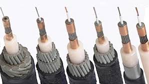
Submarine Cable Types Vary with the Level of Protection Required.
The deeper you go, the less armor protection you need to have. So deep water cables need minimal protection. Figure 6 illustrates the use of different cable types.
Figure 6: Illustration of Using Different Types of Fiber-Optic Cable.
Figures 7(a) and 7(b) show the level of fiber armor that is available. Fiber-optic cable for deep water has a size comparable to a standard garden hose (17 mm to 22 mm diameter). The armored cables can be as large as 50 mm.
Figure 7(a): Different Levels of Armor Are Used Depending on How Vulnerable the Cable is to Damage.
Figure 7(b): Cross-Section of Different Types of Submarine Cables.
Shallow water cables may need so much protection that they also must be buried.
Figure 8(a) illustrates how towed underwater plows can be used to bury cables on the sea bottom. Figure 8(b) shows a plow that can bury a fiber optic cable 2 meters under the sea bottom.
Figure 8(a): Illustration Showing How Fiber is Buried By an Underwater Plow.
Figure 8(b): Picture of Underwater Plow.
Video illustrating how a cable-laying ship deploys fiber.
These are large ships are there are multiple of them working on the ocean.
Besides laying new cable for telecommunications and fishing up old ones for repair, these ships also are busy laying fiber for sensor networks. Here is an example of a submarine fiber network, called Neptune, that services seismic sensors just off the coast of the state of Washington and British Columbia (Figure 9).
The presentation included a rough numerical example (Figure 10) of how power is fed to the cable. I am recalling this stuff from memory, but I think this is close to what was presented. I added some information about the number and power use of the repeaters because that subject interests me.
The key points of this numerical example are:
The voltage is very high (~10 kV)
The power is really not that high (~10 kW)
The distances can be enormous (thousands of kilometers)
Figure 10: Rough Power Feed Calculations.
One interesting aspect of the calculation is that a large ground difference must be accommodated between the continents. It turns out that ground level between the continents is normally low (I do not recall what low value was mentioned), but that it can get quite large (~1000 V) during geomagnetic storms (reference).
Conclusion
Sorry for the rambling nature of the post, but it represents my recollections from the talk. I wanted to make sure I wrote down the information because it was interesting.
Appendix A: Submarine Cable Power Feed Characteristics
Figure 11 shows some key specifications for a submarine cable power feed system (source).
Figure 11: Key Submarine Cable Power Feed Characteristics.
I’ve never had but one wrinkle, and I’m sitting on it.
Figure 1: A Bowhead Whale Breaches off the Coast of Western Sea of Okhotsk (Olga Shpak).
I am always surprised when I read about how long some members of the animal kingdom live. Back in 2007, I saw an article about a bowhead whale (Figure 1) that was confirmed to have lived ~130 years. In fact, there is some chemical evidence that one bowhead whale may have lived to be 211 years old.
The whale that died in 2007 was able to be more precisely aged because it had been wounded back in the 1880s by a harpoon with a specific type of harpoon head (Figure 2), which was left behind in the whale and could be dated to the 1880s. Generally, whale ages are difficult to confirm because they can only be roughly aged by protein rings that makeup the lens of the whale's eye (Figure 3).
Figure 2: 1880s Harpoon Head Found in Bowhead Whale That Died in 2007.
Figure 3: Whale Eyes Have Rings Like Trees.
Today, I saw the following graphic that shows the ages of some long-lived species (Figure 4). You can see that the bowhead whale's lifetime is just a bit more than half of the ocean quohog, a type of clam.
Figure 4: Longest Lived Animals.
There is a well-known speculation, called the Heartbeat Hypothesis, that every animal has a limited number of heartbeats – it is also called the "billion beat hypothesis" because most species seem to get ~1 billion heartbeats in a lifetime. Here is a PBS video that does a good job describing the hypothesis. The video also does a nice job explaining the quarter-power scaling principle, which some folks use to explain why larger organisms (e.g. turtles) tend to live longer than smaller ones (e.g. shrews).
The maximum longevity of a species can be quite different from the average. A great illustration of this point comes from the famous tale of Jeanne Calment, the oldest woman in history, who died at 122 years old.
One interesting story about her involved an man who wanted the rights to her apartment when she died, which is a common arrangement in France. When she was 90, the man paid 2500 francs per month for the rights to her apartment when she died. He had no idea she would outlive him. Here is a quote from the Wikipedia on the subject (see also the New York Times article on her).
In 1965, at age 90 and with no heirs, Calment signed a deal to sell her apartment to lawyer André-François Raffray, on a contingency contract. Raffray, then aged 47 years, agreed to pay her a monthly sum of 2,500 francs until she died. Raffray ended up paying Calment the equivalent of more than $180,000, which was more than double the apartment's value. After Raffray's death from cancer at the age of 77, in 1995, his widow continued the payments until Calment's death. During all these years, Calment used to say to them that she "competed with Methuselah".
He knows nothing; and he thinks he knows everything. That points clearly to a political career.
Figure 1: We are all getting older.
In a previous post, I discussed standard rules of thumb that you're told when you first look for pension advice & retirement planning. I am interested in this topic for a number of reasons:
I help my mother (who is retired) manage her money.
I am not getting any younger and I am saving for retirement.
I am encouraging my sons to save for retirement.
As I thought about it, people really need a spreadsheet that will allow them to try different retirement options – I have not been happy with any of the web-based retirement planners that I have worked with.
I have prepared a spreadsheet that allows modeling for:
Wage increases over time
Taxes and inflation while working – I do not model inflation during the retirement years.
Age you start saving and when you retire
Pension and Social Security Income
Some canned scenarios that will allow you to see examples of how it works – use Excel's Scenario Manager to see these examples
Amortization tables that show on a payment-by-payment basis how money is invested while working and expended when retired.
With this spreadsheet, I can use Excel's other functions (like Goal Seek and Solver) to experiment with different financial parameters (e.g. savings rate, rate of return) to ensure that I have a plan that will meet my objectives. Just as importantly, I can used the spreadsheet to test the sensitivity of my plan to deviations in market performance from my assumptions.
This spreadsheet was interesting to prepare because I could not use the standard Excel formulas for future value – I needed to model payments that were changing with time because of wage increases. I ended up using an array function, which did a very nice job.
The spreadsheet is here and uses no macros. You can find my previous post here.
Posted inFinancial|Comments Off on Retirement Planning Spreadsheet
Nothing in the world is worth having or worth doing unless it means effort, pain, difficulty... I have never in my life envied a human being who led an easy life. I have envied a great many people who led difficult lives and led them well.
Figure 1: Susan Oliver in The Cage (aka The Menagerie).
I just watched an excellent documentary on Susan Oliver called The Green Girl. Her iconic role was as the character Vina in the Star Trek pilot called "The Cage". Her photo in green makeup appears at the end of many episodes of the original Star Trek series (Figure 1). It appears that she had a sense of humor about all the makeup she had to wear in her role as Vina (Figure 2). I have revealed my love of all things Trek in previous posts (example), so my interest in this video should not surprise anyone.
Figure 2: Susan Oliver Clowning Around During Filming of "The Cage".
Susan Oliver was a guest star on nearly every popular show during the '60s and '70s. As she grew older, she tried to move into directing, but encountered a glass ceiling. She died in 1990 from lung cancer at 58 years old – way too young.
The documentary chronicles her life through a series of interviews with co-workers, friends, and family. The interviews include actors like David Hedison (Voyage to the Bottom of the Sea) and Lee Meriwether (Time Tunnel), both of whom starred in shows that young boys liked back in the '60s.
Susan was quite an accomplished pilot and that part of her biography was especially interesting. She wrote a book about a long-distance, single-engine, solo flight she made called Odyssey: A Daring Transatlantic Journey. I tried to buy the book, but it is frighteningly expensive. It turns out there is a very aggressive market in Susan Oliver memorabilia that has driven the price way up.
I enjoyed the documentary very much. George Pappy, the driving force behind the DVD, can be proud of his work. I will leave you with a picture of what Susan looked like without any green makeup (Figure 3).
Figure 3: Susan Oliver without Green Makeup.
In 2014, Susan was remembered with an award from the Women's International Film & Television Showcase. You can see her niece accepting the award in the following Youtube video.
I am ready to meet my Maker. Whether my Maker is prepared for the great ordeal of meeting me is another matter.
Figure 1: Secchi Disk (Wikipedia).
I have a small summer cabin on a lake in northern Minnesota that my family uses for recreation. The health of the lake is very important to me because I plan on leaving the property to my children so that my children and grandchildren (when and if they come) will have a nice place to vacation. One way to assess the health of the lake is by measuring its clarity, which is measured using a Secchi disk (Figure 1).
The Wikipedia has a good description of the disk and the measurement process, which I quote below.
The Secchi disk, as created in 1865 by Angelo Secchi, is a plain white, circular disk (30 cm in diameter or approximately 12 inches) used to measure water transparency in bodies of water. The disc is mounted on a pole or line, and lowered slowly down in the water. The depth at which the disk is no longer visible is taken as a measure of the transparency of the water.
One of the issues with measuring clarity using a Secchi disk is that the testing is performed by volunteers and the results rely on human visual judgement. In recent years, the Secchi data is being augmented with satellite water clarity data. The state of Minnesota has published a good reference paper on the topic for those of you who wish to know more.
The amount of lake data that is available today is just amazing. For example, Google provides an excellent image with a superimposed lake depth map (Figure 2). The small red area on the map is the lake's public access area.
Figure 2: Google Map of Eagle Lake in Itasca County.
The state of Minnesota provides a "Lake Finder" application that allows you to easily find information about a specific lake. To illustrate how I use the data, my cabin is on Eagle Lake and I recently downloaded the Secchi clarity data from Minnesota's web site. I then plot the data as shown in Figures 3. The plot on shows data for recent years – the data goes back into the 1980s. I will use this data in discussions with other cabin owners about the lakes health.
Figur3: Eagle Lake Secchi Disk Data.
The data is gathered by volunteers. There is no Secchi data for the months when the lake is frozen, which is indicated on the plot by the dark regions.You can see in the data that the water clarity generally improves over the winter and degrades over the summer as the amount of algae and other plants increase.
Posted inGeneral Science|Comments Off on Lake Water Clarity Over Time
A good scientist is a person with original ideas. A good engineer is a person who makes a design work with as few original ideas as possible. There are no prima donnas in engineering.
Figure 1: Laser Creating a Guide Star.
The use of adaptive optics requires that precise measurements be made of the disturbances present in the atmosphere so that they can be compensated for – a process known as deconvolution. These measurements are often made by reflecting light off of sodium atoms in the upper atmosphere. These reflections effectively create artificial stars known as guide stars (Figure 1).
The Wikipedia article on guide stars has a good description of how a sodium guide star works, which I quote here:
Sodium guide stars use laser light at 589 nm to excite sodium atoms in the mesosphere and thermosphere, which then appear to "glow". The LGS [Laser Guide Star] can then be used as a wavefront reference in the same way as a natural guide star – except that (much fainter) natural reference stars are still required for image position (tip/tilt) information. The lasers are often pulsed, with measurement of the atmosphere being limited to a window occurring a few microseconds after the pulse has been launched. This allows the system to ignore most scattered light at ground level; only light which has travelled for several microseconds high up into the atmosphere and back is actually detected.
I saw a great photo from the Gemini telescope showing the five guide star pattern it generates (Figure 2). I think this is really cool.
Figure 2: Gemini Telescope's Five Guide Star Pattern.
Posted inAstronomy|Comments Off on Cool Photo of Telescope Guide Stars
He begins working calculus problems in his head as soon as he awakens. He did calculus while driving in his car, while sitting in the living room, and while lying in bed at night.
Figure 1: Movie That Prompted a Discussion of Aspect Ratio.
I love old movies and one of the best is The Quiet Man. I recently picked up the Blu-Ray version and watched it with my wife this weekend. During the movie, my wife asked about the movie's aspect ratio – it is not a widescreen movie. The Quiet Man was filmed in Academy Ratio (1.37:1), a ratio which was standardized by the Academy of Motion Picture Arts and Sciences in 1932. The Quiet Man was released in 1952, a year before the mass introduction of a plethora of widescreen film formats.
Most of the old movies I watch are from 1953 and later, so my wife is used to seeing my old movies in widescreen format. I must admit that I love the widescreen formats and I am drawn to them for my personal viewing – I especially like VistaVision.
I thought it would be useful to review the different aspect ratios used in movies and television here. Let's begin by defining the term aspect ratio.
The aspect ratio of an image describes the proportional relationship between its width and its height. It is commonly expressed as two numbers separated by a colon, as in 16:9. For an x:y aspect ratio, no matter how big or small the image is, if the width is divided into x units of equal length and the height is measured using this same length unit, the height will be measured to be y units.
There are an enormous number of aspect ratios that have been used in motion pictures and the Wikipedia has a comprehensive list for those who are interested. I have summarized the major commercial aspect ratios in Table 1. VistaVision is still used quite a bit for movie's with special effects (e.g. Interstellar).
Table 1: List of Major Widescreen Film Formats And Aspect Ratios.
Format
Est.
Projector Aspect Ratio
Projection lenses
VistaVision
1954
1.850:1
spherical
Univisium
1998
2.000:1
spherical
Techniscope
1960
2.390:1
2x anamorphic
Technirama
1956
2.350:1
2x anamorphic
Superscope
1954
2.000:1
2x anamorphic
Super VistaVision
1989
2.210:1
spherical
Super Technirama
1959
2.210:1
spherical
Silent films
1892
1.330:1
spherical
Cinemascope
1953
2.550:1
2x anamorphic
Cinemascope
1957
2.350:1
2x anamorphic
Academy format
1932
1.370:1
spherical
Television aspect ratios are more limited and are listed as follows (source):
All content provided on the mathscinotes.com blog is for informational purposes only. The owner of this blog makes no representations as to the accuracy or completeness of any information on this site or found by following any link on this site.
The owner of mathscinotes.com will not be liable for any errors or omissions in this information nor for the availability of this information. The owner will not be liable for any losses, injuries, or damages from the display or use of this information.