
Introduction
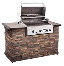
Figure 1: Gas Grill.
A friend of mine recently converted his propane-fueled grill to a natural-gas fueled grill and he mentioned to me that he had to get a new pressure regulator and different-sized gas orifice, neither of which I knew anything about. His grill looks similar to the one shown in Figure 1. He went through the conversion process with me and during this discussion I saw that the data table he used for orifice size might present me with a good demonstration of Mathcad's matrix operations. Since I am planning on offering some internal training in Mathcad in the next month or two, I thought this might be a good example for those I am training.
I do need to make a disclaimer that I am not a gas conversion professional and I am focused here on a mathematics application. See a gas conversion specialist if you need help doing a conversion.
Background
Objective
My goal here is to show how I can use Mathcad and Excel to quickly produce a useful table of results based on a formula. In fact, I will present similar data in two different ways to illustrate different approaches to the same problem. A matrix-based approach proved to be the most efficient way to generate the two table options.
Definitions
There are a few terms that I should define before we go into the details.
- drill bit sizes
- An archaic system of hole measurement still used in the United States. For more information on this topic, see this web page.
- orifice
- A small hole in the gas stream that limits the amount of gas flow. The area of the hole is a function of the required gas flow rate, gas specific gravity relative to air, and the gas pressure. Check out the Wikipedia for more details.
- specific gravity
- The density of a substance relative to a reference material, which in this case is air (see Relative Density).
- Heat of Combustion
- The amount of heat released by a specified volume of gas. Check out the Wikipedia for more details.
Grill Construction
Figure 2 shows the construction of the burner section of a typical gas grill. Observe there is an orifice that separated the gas valve from the burner. The post deals with the math behind selecting the proper orifice size for a given burner size.
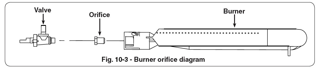
Figure 2: Basic Grill Burner Construction.
Figure 3 shows three orifices of different sizes.

Figure 3: Gas Orifices with Different Areas.
Key Formula
The key formula I will be using is shown in Equation 1 (source). This equation is an empirical relationship in that you need to use the designated units.
| Eq. 1 |  |
where
- H is the rate of heat generation [BTU/hour]
The assumption is that the grills are rated for a given heat flow and the gas conversion should leave the rate of heat generation unchanged.
- HC is the heat of combustion of the gas [BTU/ft3].
For the discussion here, I am only concerned natural gas (HC=1050 BTU/ft3) and propane (HC=2500 BTU/ft3) .
- A is the area of the orifice [in2]
The area of the orifice controls the gas flow and the rate of heat generation.
- Cd is the gas flow coefficient that is a function of the nozzle shape [unitless].
For the analysis here, I will assume that CD is 0.82. You can determine the value of the coefficient using the following chart and information about the orifice. Figure 4 shows examples of the Cd for different types of orifices and the angle of discharge.
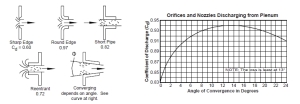
Figure 4: Coefficient of Discharge.
- h is the pressure drop across the orifice [inH2O].
For this analysis, I will assume the pressure drops from the tank pressure to atmospheric pressure.
- sg is the specific gravity of the gas relative to air at Standard Temperature and Pressure (STP) [unitless].
For this discussion, I will assume that the specific gravity of natural gas is 0.65 and of propane is 1.55. These numbers do not seem to be standardized and I have seen numerous similar, but not identical, values used.

Analysis
I will present similar information in two different formats, which I refer to as Format 1 and Format 2.
Format 1
Figure 5 shows the first format I found for the natural gas and propane orifice sizes.
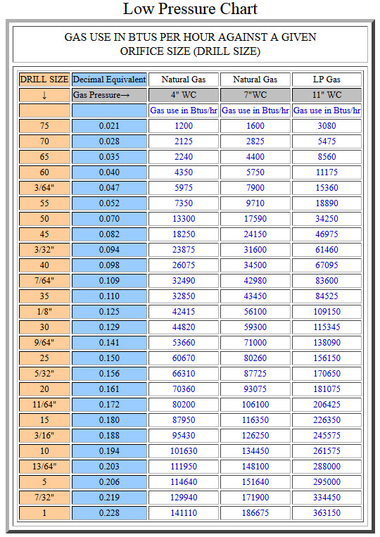
Figure 5: Table Format 1 Example.
Figure 6 shows how I generated Format 1 using Mathcad and Excel.

Figure 6: Calculation of a Table Format 1.
Format 2
Format 1 has good and bad points.
- (good – sort of) It shows you the exact heat generated for a given orifice, gas, and pressure. While I think this is a good feature, some folks may find it a useless level of detail.
- (bad) burners are usually specified in terms of even BTU values (e.g. 10,000 BTU or 20,000 BTU). Format 1 forces users to hunt for the BTU, orifice, and pressure combination they need.
I started to think about ways I could eliminate the need to hunt for the closest BTU output. Then I saw the example shown in Figure 7. I like this format because there is no hunting for the closest BTU value. I have already done that hunting using Mathcad. However, I do lose direct access to the exact heat flow value.

Figure 7: Table Format 2.
Here is how I approached generating this format.
Calculation
Figure 8 shows how I setup the calculation. The table of drill bit sizes is from the Wikipedia. The routine chooses the orifice size by computing the absolute differences from the heat generation objective and selecting the minimum.
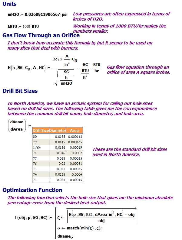
Figure 8: Table Format 2 Setup.
Figure 9 shows the actual calculation and my presentation of the table. I like to use Excel with Mathcad so that I can use its cell formatting capabilities.

Figure 9: Table Format 2 Calculation.
Error Check
Since we are working with a limited number of hole sizes, we can only approximate our desired heat output and I want to see how accurately I was able to make my desired heat flow. Figure 10 shows that my maximum error is about 7.8%, which is comparable to the variation in energy present in commercially available natural gas and propane.

Figure 10: Calculation of Heat Flow Deviation Percentages From My Objectives.
Conclusion
I was able to quickly generate tables using Mathcad and Excel that are very similar to those I found on burner conversion web sites. This should provide a good training example in matrix operations for my next training course.
Another disclaimer: This is a post about matrix operations and not burner physics. If you are converting burner fuels, go to a professional.
Here are links to the Mathcad worksheets that generate these tables.


