Introduction
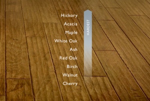
Figure 1: Wood Hardness Scale.
I have long been told that wood hardens as it ages, but I have anecdotal evidence that this is not always true. I also know that some species are far harder than others (Figure 1).
I read the following forum post that I thought presented really good information on wood hardness and moisture content that I would like to research a bit more and present here. The key point of the forum discussion was that wood gets harder as its moisture content decreases, which can happen to wood as it ages. Other factors, like insects and mold, will decrease the hardness of wood. I am only concerned with moisture here – the other factors are unpredictable.
I will present two numerical models for how the hardness of wood varies with moisture content. These two models will be shown to be roughly equivalent.
Background
Concept
There are many wood properties that vary with the moisture content of the wood. Here are a few examples:
- hardness
- shear modulus
- tensile strength
- compressive strength
I have seen two approaches to modeling the effect of moisture on these properties: (1) a power law relationship (USDA) and a linear model (Bozkurt Y, Göker Y [1987]). I will show that the two approaches produce similar results over a narrow moisture content range.
Definition of Hardness
My post here will focus on Janka hardness, which is a commonly used wood hardness measure. Here is the definition of the Janka measurement process and how moisture content is defined.
- Janka Side Hardness
- Janka side hardness is the load required to embed an 11.28-mm (0.444-in.) ball to one-half its diameter.
- Moisture Content (M)
- The percentage of wood mass consisting of water. It is often measured in the field using electrical test equipment. In the lab, it can be measured using by measuring the mass of a test sample before and after drying and computing

where
- mwater is the mass of water in the wood sample.
- mwet is the mass of the wood sample before drying.
- mdry is the mass of the dried wood sample.
Figure 2 illustrates the Janka test.

Figure 2: Illustration of the Janka Test (Wikipedia).
This post is focused on hardness, but the approach can be used for many other parameters.
Forest Products Laboratory Model (USDA)
Equation 1 shows the model from the Forest Products Laboratory (FPL). I will use data from the FPL to model wood hardness.
| Eq. 1 |
 |
where
- P a property of wood (e.g. hardness)
- P12 the property value at 12% moisture content.
- Pg is the property value under green conditions.
- M is the moisture content of the wood expressed as a percentage.
- MP is defined in Chapter 4 of the 1999 Wood Handbook as the moisture content percentage at the intersection of a horizontal line representing the strength of green wood and an inclined line representing the logarithm of the strength–moisture content relationship for dry wood. They then say to assume 25% if MP is not known. I can explain why they say assume 25% if you do not have information otherwise. The intersection statement does not seem correct. I go into detail here.
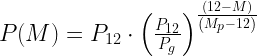
Linear Model
Equation 2 shows a model that I have seen in many publications (example, sect 2.3) for normalizing data gathered from wood at various moisture contents to 12%, which is the industry standard for moisture content.
| Eq. 2 |
![\displaystyle P\left( M \right)=\frac{{{P}_{12}}}{1+\alpha \cdot \left( M-12 \right)}\approx {{P}_{12}}\cdot \left[ 1-\alpha \cdot \left( M-12 \right) \right]](https://s0.wp.com/latex.php?latex=%5Cdisplaystyle+P%5Cleft%28+M+%5Cright%29%3D%5Cfrac%7B%7B%7BP%7D_%7B12%7D%7D%7D%7B1%2B%5Calpha+%5Ccdot+%5Cleft%28+M-12+%5Cright%29%7D%5Capprox+%7B%7BP%7D_%7B12%7D%7D%5Ccdot+%5Cleft%5B+1-%5Calpha+%5Ccdot+%5Cleft%28+M-12+%5Cright%29+%5Cright%5D&bg=ffffff&fg=000&s=2&c=20201002) |
where
- P12 is estimated value of a parameter at 12% moisture content.
- P is measured value of a parameter at a moisture content of u%.
- α is a constant that in general varies with the species of the wood under test. It can be calculated using
 . This relationship is derived in Figure 3.
Analysis
Objective
I will show how Equations 1 and 2 are related in that they produce similar results for wood hardness in the typical range of wood moisture contents.
Calculations
For my work here, I will work with the wood hardness normalized to the hardness at 12% moisture content. Normalizing allows me to work with numbers that are in the neighborhood of 1. Figure 3 shows my analysis.

Figure 3: Comparison of Exact and Linear Approximation.
Conclusion
I was able to show that Equations 1 and 2 produce similar results in the typical range of wood moisture contents (6% to 14%). I also see that the model states that wood gets harder as moisture content decreases, which is something that I have observed.
To centralize the data that I use for my personal work, I have included a list of the hardness parameters for common North American Species (Table 1).
Appendix A: MP Values for Common North American Species.
MP is an important parameter for estimating wood hardness and its value varies by species. The Wood Handbook states that its value is normally near 25%. Figure 4 shows some common MP values and you can see that they are near 25%.

Figure 4: Table 4-13 from the Wood Handbook.
Appendix B: MP Definition Discussion.
The definition of Equation 1 includes some phrasing that is difficult for me to figure out. I will try to provide some additional clarification here. Here is how MP is defined.
MP [is the] moisture content at the intersection of a horizontal line representing the strength of green wood and an inclined line representing the logarithm of the strength–moisture content relationship for dry wood.
I actually could not understand this statement as written, although I do think I can explain how you determine MP. Figure 5 shows my explanation, which assumes you have (1) a plot of the hardness versus moisture content of the wood in question, and (2) you know the green hardness.

Figure 5: Explanation for Mp Determination Statement.
Figure 5 shows that the if we graph Equation 1, MP is the moisture level at which the wood strength equals the green strength. Figure 6 illustrates the relationship between MP and the Fiber Saturation Point (FSP). Observe that the "green" strength is reached before the FSP. This means that Equation 2 does not hold above MP.

Figure 6: Relationship Between Mp and FSP.
Appendix C: Table of Hardness Values (Dry/Green/Ratio) for Common Species.
Table 1 is from a US Forest Service publication, which I have augmented with a column of common tree names. The scientific names are not of much use for me – I only know the common names of trees. Note that the hardness levels are specified in units of Newtons (metric measure) and there are 4.448 Newtons in a pound. For example, the hardness of Black Cherry is rated at 4210 Newtons, which is ~950 pounds.
Table 1: Hardness (Dry/Green) and Dry/Green Ratio By Species
| Type |
Common Name |
Species |
Dry Hard. (N) |
Green Hard. (N) |
Dry/Green Ratio |
| Hardwood |
ALDER, COMMON |
ALNUS GLUTINOSA |
2940 |
2220 |
1.32 |
|
ALDER, RED |
ALNUS RUBRA |
2620 |
1950 |
1.34 |
|
ASH, BLACK |
FRAXINUS NIGRA |
3770 |
2310 |
1.63 |
|
ASH, EUROPEAN |
FRAXINUS EXCELSIOR |
6140 |
4270 |
1.44 |
|
ASH, GREEN |
FRAXINUS PENNSYLVANICA |
5320 |
3860 |
1.38 |
|
ASH, OREGON |
FRAXINUS LATIFOLIA |
5140 |
3500 |
1.47 |
|
ASH, WHITE |
FRAXINUS AMERICANA |
5850 |
4260 |
1.37 |
|
ASPEN, QUAKING |
POPULUS TREMULOIDES |
1550 |
1330 |
1.17 |
|
BEECH, AMERICAN |
FAGUS GRANDIFOLIA |
5760 |
3770 |
1.53 |
|
BEECH, EUROPEAN |
FAGUS SYLVATICA |
6410 |
4270 |
1.50 |
|
BIRCH, BLACK |
BETULA LENTA |
6520 |
4300 |
1.52 |
|
BIRCH, PAPER |
BETULA PAPYRIFERA |
4040 |
2480 |
1.63 |
|
BIRCH, YELLOW |
BETULA ALLEGHANIENSIS |
5590 |
3460 |
1.62 |
|
BUTTERNUT |
JUGLANS CINEREA |
2170 |
1730 |
1.25 |
|
CHERRY, BLACK |
PRUNUS SEROTINA |
4210 |
2930 |
1.44 |
|
CHERRY, SWEET |
PRUNUS AVIUM |
5780 |
4140 |
1.40 |
|
CHESTNUT, AMERICAN |
CASTANEA DENTATA |
2390 |
1860 |
1.28 |
|
CHESTNUT, SWEET |
CASTANEA SATIVA |
3070 |
3160 |
0.97 |
|
COTTONWOOD, BLACK |
POPULUS TRICHOCARPA |
1550 |
1110 |
1.40 |
|
COTTONWOOD, EASTERN |
POPULUS DELTOIDES |
1910 |
1510 |
1.26 |
|
CUCUMBERTREE |
MAGNOLIA ACUMINATA |
3100 |
2310 |
1.34 |
|
GUM, BLACK |
NYSSA SYLVATICA |
3590 |
2840 |
1.26 |
|
HACKBERRY, NORTHERN |
CELTIS OCCIDENTALIS |
3900 |
3100 |
1.26 |
|
HONEYLOCUST |
GLEDITSIA TRIACANTHOS |
7010 |
6160 |
1.14 |
|
HORNBEAM, EUROPEAN |
CARPINUS BETULUS |
6980 |
5470 |
1.28 |
|
HORSE CHESTNUT |
AESCULUS HIPPOCASTANUM |
3340 |
2580 |
1.29 |
|
MAGNOLIA, SOUTHERN |
MAGNOLIA GRANDIFLORA |
4520 |
3280 |
1.38 |
|
MAPLE, BIGLEAF |
ACER MACROPHYLLUM |
3770 |
2750 |
1.37 |
|
MAPLE, BLACK |
ACER NIGRUM |
5230 |
3730 |
1.40 |
|
MAPLE, RED |
ACER RUBRUM |
4210 |
3100 |
1.36 |
|
MAPLE, SILVER |
ACER SACCHARINUM |
3100 |
2620 |
1.18 |
|
MAPLE, SUGAR |
ACER SACCHARUM |
6430 |
4300 |
1.50 |
|
MAPLE, SYCAMORE |
ACER PSEUDOPLATANUS |
4850 |
3830 |
1.27 |
|
OAK, AUSTRIAN |
QUERCUS CERRIS |
8270 |
6180 |
1.34 |
|
OAK, SCARLET |
QUERCUS COCCINEA |
6210 |
5320 |
1.17 |
|
OAK, SWAMP WHITE |
QUERCUS BICOLOR |
7180 |
5140 |
1.40 |
|
OAK, WHITE |
QUERCUS ALBA |
6030 |
4700 |
1.28 |
|
PECAN |
CARYA ILLINOENSIS |
8070 |
5810 |
1.39 |
|
PLANETREE, LONDON |
PLATANUS ACERIFOLIA |
5650 |
4270 |
1.32 |
|
POPLAR, TULIP |
LIRIODENDRON TULIPIFERA |
2390 |
1950 |
1.23 |
|
SWEETGUM |
LIQUIDAMBAR STYRACIFLUA |
3770 |
2660 |
1.42 |
|
SYCAMORE |
PLATANUS OCCIDENTALIS |
3410 |
2710 |
1.26 |
|
TUPELO, WATER |
NYSSA AQUATICA |
3900 |
3150 |
1.24 |
|
WALNUT, BLACK |
JUGLANS NIGRA |
4480 |
3990 |
1.12 |
|
WALNUT, PERSIAN |
JUGLANS REGIA |
3600 |
2970 |
1.21 |
|
POPLAR, CANADIAN |
POPULUS CANADENSIS |
2220 |
2050 |
1.08 |
|
POPLAR, SILVER |
POPULUS CANESCENS |
2360 |
1730 |
1.36 |
Hardwood
Average |
|
|
4474 |
3343 |
1.34 |
| Softwood |
BALDCYPRESS |
TAXODIUM DISTICHUM |
2260 |
1730 |
1.31 |
|
CEDAR, ALASKA |
CHAMAECYPARIS OOTKATENSIS |
2570 |
1950 |
1.32 |
|
CEDAR, ATLANTIC WHITE |
CHAMAECYPARIS THYOIDES |
1550 |
1290 |
1.20 |
|
CEDAR, PORT ORFORD |
CHAMAECYPARIS LAWSONIANA |
2790 |
1690 |
1.65 |
|
FIR, BALSAM |
ABIES BALSAMEA |
1770 |
1290 |
1.37 |
|
FIR, CALIFORNIA RED |
ABIES MAGNIFICA |
2220 |
1600 |
1.39 |
|
FIR, DOUGLAS |
PSEUDOTSUGA MENZIESII |
2930 |
2260 |
1.30 |
|
FIR, GRAND |
ABIES GRANDIS |
2170 |
1600 |
1.36 |
|
FIR, NOBLE |
ABIES PROCERA |
1820 |
1290 |
1.41 |
|
FIR, PACIFIC SILVER |
ABIES AMABILIS |
1910 |
1380 |
1.38 |
|
FIR, SILVER |
ABIES ALBA |
2850 |
1910 |
1.49 |
|
FIR, SUBALPINE |
ABIES LASIOCARPA |
1550 |
1150 |
1.35 |
|
FIR, WHITE |
ABIES CONCOLOR |
2130 |
1510 |
1.41 |
|
HEMLOCK, EASTERN |
TSUGA CANADENSIS |
2220 |
1770 |
1.25 |
|
HEMLOCK, MOUNTAIN |
TSUGA MERTENSIANA |
3020 |
2080 |
1.45 |
|
HEMLOCK, WESTERN |
TSUGA HETEROPHYLLA |
2390 |
1820 |
1.31 |
|
INCENSE CEDAR |
LIBOCEDRUS DECURRENS |
2080 |
1730 |
1.20 |
|
LARCH, EUROPEAN |
LARIX DECIDUA |
3770 |
2450 |
1.54 |
|
LARCH, JAPANESE |
LARIX KAEMPFERI |
2940 |
2140 |
1.37 |
|
LARCH, WESTERN |
LARIX OCCIDENTALIS |
3680 |
2260 |
1.63 |
|
PINE, AUSTRIAN |
PINUS NIGRA |
2890 |
1910 |
1.51 |
|
PINE, CLUSTER |
PINUS PINASTER |
2670 |
1690 |
1.58 |
|
PINE, EASTERN WHITE |
PINUS STROBUS |
1690 |
1290 |
1.31 |
|
PINE, JACK |
PINUS BANKSIANA |
2530 |
1770 |
1.43 |
|
PINE, LOBLOLLY |
PINUS TAEDA |
3060 |
2000 |
1.53 |
|
PINE, LODGEPOLE |
PINUS CONTORTA |
2130 |
1460 |
1.46 |
|
PINE, LONGLEAF |
PINUS PALUSTRIS |
3860 |
2620 |
1.47 |
|
PINE, MONTEREY |
PINUS RADIATA |
3330 |
2130 |
1.56 |
|
PINE, PONDEROSA |
PINUS PONDEROSA |
2040 |
1420 |
1.44 |
|
PINE, RED |
PINUS RESINOSA |
2480 |
1510 |
1.64 |
|
PINE, SCOTCH |
PINUS SYLVESTRIS |
2980 |
2220 |
1.34 |
|
PINE, SHORTLEAF |
PINUS ECHINATA |
3060 |
1950 |
1.57 |
|
PINE, SPRUCE |
PINUS GLABRA |
2930 |
2000 |
1.47 |
|
PINE, SUGAR |
PINUS LAMBERTIANA |
1690 |
1200 |
1.41 |
|
PINE, VIRGINIA |
PINUS VIRGINIANA |
3280 |
2390 |
1.37 |
|
PINE, WESTERN WHITE |
PINUS MONTICOLA |
1860 |
1150 |
1.62 |
|
REDCEDAR, EASTERN |
JUNIPERUS VIRGINIANA |
4000 |
2880 |
1.39 |
|
REDCEDAR, WESTERN |
THUJA PLICATA |
1550 |
1150 |
1.35 |
|
REDWOOD, COAST |
SEQUOIA SEMPERVIRENS |
2130 |
1820 |
1.17 |
|
SPRUCE, BLACK |
PICEA MARIANA |
2310 |
1640 |
1.41 |
|
SPRUCE, ENGELMANN |
PICEA ENGELMANNII |
1730 |
1150 |
1.50 |
|
SPRUCE, NORWAY |
PICEA ABIES |
2110 |
1420 |
1.49 |
|
SPRUCE, RED |
PICEA RUBENS |
2170 |
1550 |
1.40 |
|
SPRUCE, SERBIAN |
PICEA OMORIKA |
2710 |
1470 |
1.84 |
|
SPRUCE, SITKA |
PICEA SITCHENSIS |
2260 |
1550 |
1.46 |
|
TAMARACK |
LARIX LARICINA |
2620 |
1690 |
1.55 |
|
WHITE CEDAR, NORTHERN |
THUJA OCCIDENTALIS |
1420 |
1020 |
1.39 |
Softwood
Average |
|
|
2470 |
1722 |
1.43 |
| Grand Average |
|
|
3472 |
2533 |
1.38 |


 , where T is the wood temperature.
 , where


 , where M is the moisture percentage, "30" represents the assumed moisture content of green wood (30%), and L% is the percentage change in length. This is Equation 3-4 in the


