Introduction

Figure 1: Example of Low-Landscape Lighting.
I have a beautiful new decking thanks to the guys at Composite Decking Boards | WPC Plastic Decking | UK Supplier and my backyard is looking better than ever, but it's not quite finished. I want some lighting out there and I have a small low-voltage lighting project in mind, similar to what shows in Figure 1 - though I did consider going for a Lampadaire exterieur, or outdoor lamp post first, after seeing them in people's gardens I'm fond of the low-level light the ones in Figure 1 show. I think they look so minimalist yet effective. I have not done a significant low-voltage wiring project in quite a few years, so I decided to do a bit of reading. It's quite a big project for a beginner so I wanted to do plenty of research to ensure I didn't make any mistakes. This comprehensive buyer's guide helped me learn more about which lighting to get and I've also watched lots of YouTube videos so that I can learn about installation. In one of the light vendor's manuals, I saw a table of allowed wattages for lighting as a function of distance and wire diameter. I thought it would be a useful exercise for me to duplicate the results shown in this table to confirm that I understand how the wiring works. This provides me some empirical verification that my "code" is correct.
While this is just a simple application of Ohm's law, it does a nice job of illustrating how to use a computer algebra system (Mathcad) to solve this type of problem. It also illustrates how even simple problems involve assumptions and approximations.
Many low-voltage wiring installation manuals include a table of allowed wattages as a function of wiring distances and wire gauge. I noticed that they are nearly all different. As I looked at the various tables, it appears that each table assumes a specific lamp layout (be it a photo moon lamp or other kind) – a layout that is often not named. I thought I would examine one of these tables in detail to see if I really understood what is going on. This post summarizes this analysis work.
Most of the installation manuals are still written assuming a halogen bulb. Outdoor LED fixtures are just starting to become common. While my work here will focus on the duplicating the results of a halogen bulb-based table, but it can easily be extended to be applicable for LED fixtures.
Background
Objective
The light level from a halogen bulb is strongly dependent on the voltage across the bulb and I want all the bulbs to have roughly the same level of brightness. Figure 2 illustrates the impact of voltage on light output (source). My design objective is to ensure that the voltages in the system are within 5% of each other, which means that light outputs should be within 80% of their nominal values.

Figure 2: % Luminous Output Versus % Design Voltage.
Load Assumptions
I needed to make a number of assumptions to create a simple model:
- These systems are referred to as "12 V", but the transformers that drive them often have taps for other voltages ? 12 V, 13 V, 14 V, 15 V taps are commonly seen. I will perform my analysis with the 13 V tap.
Most of the tables appear to use the 12 V tap, but the table I am working with here appeared to use the 14 V tap.
- All lamps are 12 V halogen.
There are LED lights available, but most of the design manuals are still targeted for halogen lights.
- The lamps are all equally spaced and we will model their load as a point load mid-way along the lamp run.
All the wiring tables I have seen appear to assume that the bulbs are arranged in a perfectly regular pattern.
- We are going to limit the amount of voltage variation between bulbs to 5% of the input voltage.
I have seen tables use voltage tolerance between 5% and 15%. The brightness of halogen bulbs is quite sensitive to the voltage applied to them – a 15% drop in voltage can result in a 50% reduction in light output (lumens).
Circuit Configuration
Figure 3 shows the schematic of the circuit that represents the low-voltage circuit discussed in the reference installation guide. I model the voltage drop for the distributed current load as if the all the current was sunk at the mid-point of the wire segment. I justify this approximation in Appendix A. You could also model it as half the total current was dissipated at the end of the wire segment.
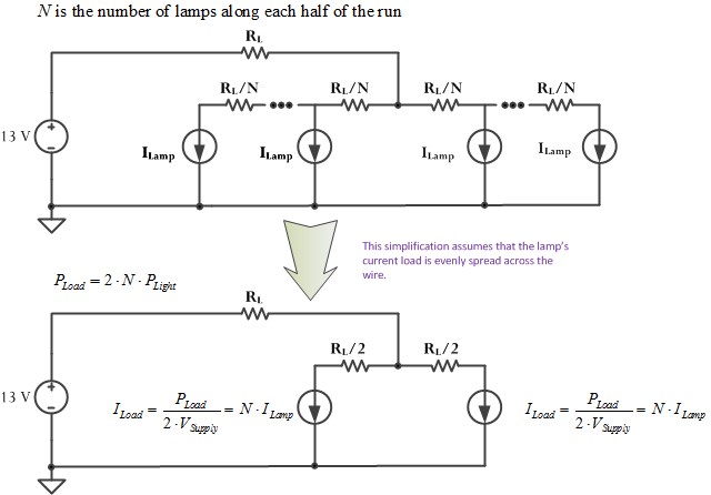
Figure 3: Schematic of My Low-Voltage Lamp Circuit Model.
- The total length of the wire run of lamps is L feet, which has a resistance of RL ?.
This is a reasonable approach to designing this type of circuit.
- The power is fed into the center of the run of lamps.
This feed configuration reduces the voltage drop over driving the all the lamps in series.
- Each lamp is modeled as a current sink.
While a voltage-variable resistance would be more accurate, we are not going to allow the voltage across any lamp to be more than 5% different than any other point in the circuit. This means that the lamp resistance will not vary by much.
- The center of lamp run is fed by a wire of the same length as the total lamp run, which is 2L feet, which means there are L feet of lamps on either side of the center-feed.
You need to make some assumption as to how the voltage gets to the run of lamps.
Analysis
Reference Table
Figure 4 shows the reference table that I will be using for my design reference. It comes from this installation guide.

Figure 4: Reference Wiring Table.
Cable Resistance Versus American Wire Gauge
While I dislike using archaic units, all the wire at my local hardware store is sold with diameters specified in AWG and I have to use these units. I will proceed in two steps: (1) create a function to compute the resistivity of copper versus AWG, (2) model the resistance of copper wire using the copper resistivity function and its length and temperature.
Figure 5 shows my resistivity function. I have used this function for years and I forget where I got the data used in it. The units in it are atrocious - ?/m versus AWG. However, I have verified its correctness numerous times.

Figure 5: Copper Resistivity Versus AWG.
Figure 6 shows my cable resistance function with length, AWG, and temperature as input variables. The function includes the a table that describes how the resistivity of copper varies with temperature. The function is so old that I do not remember where I got this data, but I have used it in many applications before and it has been compared with other sources.

Figure 6: Mathcad Formula for the Resistance of Cable In Terms of Length, AWG, and Temperature.
Calculations
My model makes some simplifying assumptions:
- Wire power losses are small enough to be ignorable ? all power is lost in the bulbs.
- All bulbs use the same amount of power.
- The lamps are connected to the 13 V tap.
Figure 7 shows my calculations for duplicating the reference table (Figure 3).

Figure 7: My Version of the Reference Table.
This table contains very similar numbers to the reference table ? the differences are probably due to minor deviations between our models for the resistivity of copper.
Conclusion
I was able to duplicate the results in the reference table, so I think I understand how to determine the voltage drops in a simple low-voltage network. My layout will be different than this simple center-fed, single-run design. However, the design principles will be identical and I will use this model to ensure that my voltages are within my specifications.
Appendix A: Justification for Voltage Drop Approximation
Figure 8 shows how we can approximate the voltage drop across one lighting segment by assuming the total line current is sunk at the mid-point of the segment off the center-feed.

Figure 8: Justification for Use of Voltage Drop Approximation.

 One of my favorite old movies is the "The African Queen" with Humphrey Bogart (he played Charlie) and Katherine Hepburn (she played Rose). In that movie, Rose asks Charlie "Could you make a torpedo?" and Charlie responds:


 . I would interpret this to mean that your cost risk is 20% of the projects estimated overall cost. This number seems to conform to my own experience with home remodeling projects. All of these projects incur some sort of unpredictable variation. In the best cases, I would estimate that they typically run ~20% over budget. In the worst case, I have had remodeling projects cost twice what I expected.
 - she had no reasons to suspect a major cost overrun. Note that there was significant material cost involved in this system and the DP model ignores it.
 - a doubling of the project cost. Unfortunately, this number is probably about right.
![\displaystyle {{\alpha }_C}=\frac{\frac{20\cdot \log \left( e \right)}{2\cdot \text{138 }\!\!\Omega\!\!\text{ }}}{\log \left( \frac{D}{d} \right)}\cdot \sqrt{\frac{f\cdot {{\mu }_{0}}\cdot {{\epsilon }_{0}}}{\pi }}\cdot \left( \frac{\sqrt{{{\rho }_{O}}.{{\mu }_{R}}}}{D}+\frac{\sqrt{{{\rho }_{I}}\cdot {{\mu }_{R}}}}{d} \right)\text{ }\left[ \frac{\text{dB}}{m} \right]](https://s0.wp.com/latex.php?latex=%5Cdisplaystyle+%7B%7B%5Calpha+%7D_C%7D%3D%5Cfrac%7B%5Cfrac%7B20%5Ccdot+%5Clog+%5Cleft%28+e+%5Cright%29%7D%7B2%5Ccdot+%5Ctext%7B138+%7D%5C%21%5C%21%5COmega%5C%21%5C%21%5Ctext%7B+%7D%7D%7D%7B%5Clog+%5Cleft%28+%5Cfrac%7BD%7D%7Bd%7D+%5Cright%29%7D%5Ccdot+%5Csqrt%7B%5Cfrac%7Bf%5Ccdot+%7B%7B%5Cmu+%7D_%7B0%7D%7D%5Ccdot+%7B%7B%5Cepsilon+%7D_%7B0%7D%7D%7D%7B%5Cpi+%7D%7D%5Ccdot+%5Cleft%28+%5Cfrac%7B%5Csqrt%7B%7B%7B%5Crho+%7D_%7BO%7D%7D.%7B%7B%5Cmu+%7D_%7BR%7D%7D%7D%7D%7BD%7D%2B%5Cfrac%7B%5Csqrt%7B%7B%7B%5Crho+%7D_%7BI%7D%7D%5Ccdot+%7B%7B%5Cmu+%7D_%7BR%7D%7D%7D%7D%7Bd%7D+%5Cright%29%5Ctext%7B+%7D%5Cleft%5B+%5Cfrac%7B%5Ctext%7BdB%7D%7D%7Bm%7D+%5Cright%5D&bg=ffffff&fg=000&s=2&c=20201002)
 is the
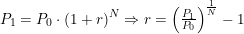
  . So I can restate Equation 1 as shown in Equation 2.