The Legend of the Management Cookies

Figure 1: Management Cookies.

Figure 1: Management Cookies.

I love having young engineers on my team. I also love cookies and we occasionally have cookies at some of our meetings – people might not attend otherwise, including me. However, our cookie selection is generally not particularly inspired.

One day was different. For a meeting of managers, someone stopped by a bakery and bought some serious cookies (Figure 1). Far more cookies were bought than the managers could eat and, after the meeting, the excess cookies were placed in our lunch room for anyone to eat. One of our young engineers, seeing the plate of exceptional cookies, exclaimed, "Where did these cookies come from?" The manager who placed the plate of cookies in the lunch room was standing near this young lad and said, with a straight face, "Those are management cookies."

Figure 2: Oliver Asking For More.

Figure 2: Oliver Asking For More.

A sad look came over the young engineer's his face and he asked very seriously, "Can I have some management cookies?" We all broke out laughing. He sounded like the title character in "Oliver Twist" asking "Please, sir, I want some more".

Now, whenever we have cookies there is always someone who asks, "Are they management cookies?"

Posted in Humor, Management | Comments Off on The Legend of the Management Cookies

Interesting Discussion on Lithium Battery Fire Hazard

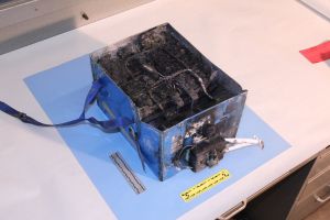
Lithium-Cobalt Batteries After Dreamliner Fire.

Dreamliner APU After Lithium-Cobalt Battery Fire.

We have all heard stories of the  fire hazards that lithium-ion batteries present – just to remind you, here is a partial list:

There have been many other documented "thermal events". I personally have seen a lithium-ion battery catch fire on an engineer's bench and it was impressive.

One of the hazardous aspects of many lithium chemistries involves the flammability of their electrolyte (source):

Lithium-ion batteries can be dangerous under some conditions and can pose a safety hazard since they contain, unlike other rechargeable batteries, a flammable electrolyte and are also kept pressurized.

There are numerous discussions of the flammability of lithium-ion batteries on the web (example). While I understand how a lithium-ion battery can burn, I have never had a good understanding of how the fire can initiate.

Today, I saw this article and it gave a very good description of how a lithium-ion battery can be "encouraged" to catch fire. Here is the key quote:

A typical lithium-ion battery consists of two tightly packed electrodes – a carbon anode and a lithium metal-oxide cathode – with an ultrathin polymer separator in between. The separator keeps the electrodes apart. If it's damaged, the battery could short-circuit and ignite the flammable electrolyte solution that shuttles lithium ions back and forth.

"The separator is made of the same material used in plastic bottles," said graduate student Denys Zhuo, co-lead author of the study. "It's porous so that lithium ions can flow between the electrodes as the battery charges and discharges."

Manufacturing defects, such as particles of metal and dust, can pierce the separator and trigger shorting, as Sony discovered in 2006. Shorting can also occur if the battery is charged too fast or when the temperature is too low – a phenomenon known as overcharge.

"Overcharging causes lithium ions to get stuck on the anode and pile up, forming chains of lithium metal called dendrites," Cui explained. "The dendrites can penetrate the porous separator and eventually make contact with the cathode, causing the battery to short."

Dendrite formation causing trouble does not surprise me – I have had to deal with dendrites in other contexts (e.g. salt dendrites that formed across battery poles that were inadvertently exposed to sea water) and it is amazing how destructive they can be.

In case you are wondering why there is a separator in the battery, take a look in the Wikipedia under salt bridge.

Here is an FAA video on dealing with laptop battery fires that shows an actual laptop fire at LAX  at the beginning of the video.

Posted in Batteries, Electronics | 1 Comment

Network Data rates: Advertised Versus Actual

Introduction

Figure 1: Typical Usage Model for HPNA.

Figure 1: Typical Usage Model for HPNA.

I often get questions from customers on what data rate can they expect from their particular network protocol, like Ethernet, MoCA, or HPNA. They often have expectations that have been set by marketing material and not reality. I thought it would be worthwhile reviewing what drives the effective data rate of typical network protocol and how that number differs from what is often reported in the product's marketing material.

There are no doubts about it, internet and telephone networks have never been more important. This is particularly true for businesses such as IT companies in Melbourne and all over the world that rely on their IT networks to keep in touch with their customers. Above all, maintaining an open communication channel is the key to success for companies that operate from an online platform.

That being said, for my example, I will use the Home Phone Network Alliance (HPNA) standard, which is commonly used to distribute data over old phone lines (twisted pair) and coaxial cable (Figure 1). For this discussion, I will not need to go into the HPNA's operational details – we are going to focus on the definitions of a few terms that are commonly used to describe data rates. As usual, the answer becomes complicated because the data rate you obtain is a function of the version of integrated circuit you are using.

Understanding bit rates for a network is similar to trying to understand the gas mileage numbers for a car. The car manufacturers emphasize the highway mileage numbers, which are optimistic and that few, if any, drivers obtain. The city driving numbers probably are closer to what most drivers will get, but even these numbers are frequently optimistic. The actual mileage depends strongly on how you drive – same with network performance. You can do configuration via an Arris router login to fine tune the engine of the connection that is the router, which can help up the speed (or the mileage), but before doing so it is important to understand what the ISP means by data rate.

Background

There are three common terms used to specify data rate:

Theoretical Physical Rate (TPR)
The total number of bits transferred per second. This parameter ignores the overheads associated with forming bits into packets, managing these packet, and dealing with errors.
Errors and malfunctioning networks can sometimes lead to data loss in the computer systems that run them. In such situations, Storage Area Network (SAN) data recovery and similar services can be utilized by administrators to restore the data.
Practical Physical Rate (PPR)
The total number of bits transferred per second after handling errors.
Data Rate (DR)
The actual number of data bits transferred per second after removing the overheads associated with transport overheads like Internet Protocol (IP).

I often have customers tell me that they expected the TPR because of what they had read in marketing material, but they measured the DR, which is often not listed. I will use HPNA as an example of how these three specifications are related.

Analysis

TPR Calculation

Equation 1 shows how the TPR is computed, which is of interest to hardware designers because it drives the performance requirements for their part of the network. This is the number I usually hear customers repeating. They will NEVER obtain this rate in practice.

Eq. 1 \displaystyle {{R}_{TPR}}={{N}_{Symbol}}\cdot {{f}_{Symbol}}

where

  • NSymbol is the number of bits per symbol.
  • fSymbol is the rate of symbol transmission.

PPR Calculation

Equation 2 shows how the PPR is computed, which is mainly of interest to hardware developers who are dealing with the error-correcting portions of the system. I do not hear this number from customers much, but it has come up – customers will never obtain this rate in practice either.

Eq. 2 \displaystyle {{\left. {{R}_{PRR}}={{N}_{Symbol}} \right|}_{\text{Packet }\!\!~\!\!\text{ Error }\!\!~\!\!\text{ Rate }\!\!~\!\!\text{ }=1\text{E}-7}}\cdot {{f}_{Symbol}}

where

  • N is the HPNA overhead for supporting IP.

DR Calculation

Equation 3 shows how the DR is computed. The customers actually have a chance at obtaining this number, assuming all is going smoothly. It is comparable to the city driving number for gas mileage.

Eq. 3 {{R}_{Data}}={{R}_{PRR}}\cdot (1-k)

where

  • k is the HPNA overhead for supporting IP.

Calculations

TPR

Table 2: Practical Physical Rates for Each of the HPNA Chip Sets
Chip Version fSymbol (Mbps) NSymbol (bits) PPR (Mbps)
CCG3010 16 10 160
CCG3110 16 10 160
CCG3210 32 10 320

PPR

Table 2: Practical Physical Rates for Each of the HPNA Chip Sets
Chip Version fSymbol (Mbps) NSymbol|1E-7 (bits) PPR (Mbps)
CCG3010 16 7 112
CCG3110 16 9 144
CCG3210 32 8 256

DR

I have actually had customers obtain the rates shown in Table 3. However, those rates were obtained in an almost ideal test environment. Start adding multiple data interfaces and the rates begin to drop because of other system overheads associated with multiple interfaces vying for the shared media.

Table 3: Data Rates for Each of the HPNA Chip Sets
Chip Version PPR (Mbps) Overhead Data Rate (Mbps)
CCG3010 112 27% 81.8
CCG3110 144 27% 105.1
CCG3210 256 27% 186.9

Conclusion

This question came up today and I thought my response was worth documenting here.

Posted in Electronics | 1 Comment

A Small Low-Voltage Landscape Wiring Project

Introduction

Figure 1: Example of Low-Landscape Lighting.Figure 1: Example of Low-Landscape Lighting.


Figure 1: Example of Low-Landscape Lighting.

I have a beautiful new decking thanks to the guys at Composite Decking Boards | WPC Plastic Decking | UK Supplier and my backyard is looking better than ever, but it's not quite finished. I want some lighting out there and I have a small low-voltage lighting project in mind, similar to what shows in Figure 1 - though I did consider going for a Lampadaire exterieur, or outdoor lamp post first, after seeing them in people's gardens I'm fond of the low-level light the ones in Figure 1 show. I think they look so minimalist yet effective. I have not done a significant low-voltage wiring project in quite a few years, so I decided to do a bit of reading. It's quite a big project for a beginner so I wanted to do plenty of research to ensure I didn't make any mistakes. This comprehensive buyer's guide helped me learn more about which lighting to get and I've also watched lots of YouTube videos so that I can learn about installation. In one of the light vendor's manuals, I saw a table of allowed wattages for lighting as a function of distance and wire diameter. I thought it would be a useful exercise for me to duplicate the results shown in this table to confirm that I understand how the wiring works. This provides me some empirical verification that my "code" is correct.

While this is just a simple application of Ohm's law, it does a nice job of illustrating how to use a computer algebra system (Mathcad) to solve this type of problem. It also illustrates how even simple problems involve assumptions and approximations.

Many low-voltage wiring installation manuals include a table of allowed wattages as a function of wiring distances and wire gauge. I noticed that they are nearly all different. As I looked at the various tables, it appears that each table assumes a specific lamp layout (be it a photo moon lamp or other kind) – a layout that is often not named. I thought I would examine one of these tables in detail to see if I really understood what is going on. This post summarizes this analysis work.

Most of the installation manuals are still written assuming a halogen bulb. Outdoor LED fixtures are just starting to become common. While my work here will focus on the duplicating the results of a halogen bulb-based table, but it can easily be extended to be applicable for LED fixtures.

Background

Objective

The light level from a halogen bulb is strongly dependent on the voltage across the bulb and I want all the bulbs to have roughly the same level of brightness. Figure 2 illustrates the impact of voltage on light output (source). My design objective is to ensure that the voltages in the system are within 5% of each other, which means that light outputs should be within 80% of their nominal values.

Figure 2: % Luminous Output Versus Percent Design Voltage.

Figure 2: % Luminous Output Versus % Design Voltage.

Load Assumptions

I needed to make a number of assumptions to create a simple model:

  • These systems are referred to as "12 V", but the transformers that drive them often have taps for other voltages ? 12 V, 13 V, 14 V, 15 V taps are commonly seen. I will perform my analysis with the 13 V tap.

    Most of the tables appear to use the 12 V tap, but the table I am working with here appeared to use the 14 V tap.

  • All lamps are 12 V halogen.

    There are LED lights available, but most of the design manuals are still targeted for halogen lights.

  • The lamps are all equally spaced and we will model their load as a point load mid-way along the lamp run.

    All the wiring tables I have seen appear to assume that the bulbs are arranged in a perfectly regular pattern.

  • We are going to limit the amount of voltage variation between bulbs to 5% of the input voltage.

    I have seen tables use voltage tolerance between 5% and 15%. The brightness of halogen bulbs is quite sensitive to the voltage applied to them – a 15% drop in voltage can result in a 50% reduction in light output (lumens).

Circuit Configuration

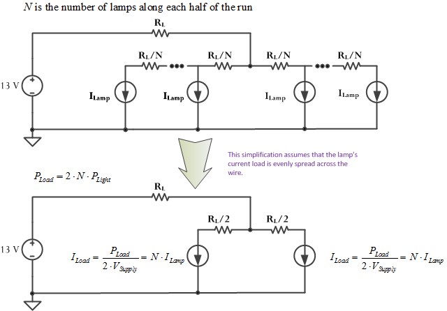
Figure 3 shows the schematic of the circuit that represents the low-voltage circuit discussed in the reference installation guide. I model the voltage drop for the distributed current load as if the all the current was sunk at the mid-point of the wire segment. I justify this approximation in Appendix A. You could also model it as half the total current was dissipated at the end of the wire segment.

Figure 3: Schematic of My Low-Voltage Lamp Circuit Model.

Figure 3: Schematic of My Low-Voltage Lamp Circuit Model.

  • The total length of the wire run of lamps is L feet, which has a resistance of RL ?.

    This is a reasonable approach to designing this type of circuit.

  • The power is fed into the center of the run of lamps.

    This feed configuration reduces the voltage drop over driving the all the lamps in series.

  • Each lamp is modeled as a current sink.

    While a voltage-variable resistance would be more accurate, we are not going to allow the voltage across any lamp to be more than 5% different than any other point in the circuit. This means that the lamp resistance will not vary by much.

  • The center of lamp run is fed by a wire of the same length as the total lamp run, which is 2L feet, which means there are L feet of lamps on either side of the center-feed.

    You need to make some assumption as to how the voltage gets to the run of lamps.

Analysis

Reference Table

Figure 4 shows the reference table that I will be using for my design reference. It comes from this installation guide.

Figure 3: Reference Wiring Table.

Figure 4: Reference Wiring Table.

Cable Resistance Versus American Wire Gauge

While I dislike using archaic units, all the wire at my local hardware store is sold with diameters specified in AWG and I have to use these units. I will proceed in two steps: (1) create a function to compute the resistivity of copper versus AWG, (2) model the resistance of copper wire using the copper resistivity function and its length and temperature.

Figure 5 shows my resistivity function. I have used this function for years and I forget where I got the data used in it. The units in it are atrocious - ?/m versus AWG. However, I have verified its correctness numerous times.

Figure 4: Copper Resistivity Versus AWG.

Figure 5: Copper Resistivity Versus AWG.

Figure 6 shows my cable resistance function with length, AWG, and temperature as input variables. The function includes the a table that describes how the resistivity of copper varies with temperature. The function is so old that I do not remember where I got this data, but I have used it in many applications before and it has been compared with other sources.

Figure 4: Mathcad Formula for the Resistance of Cable In Terms of Length, AWG, and Temperature.

Figure 6: Mathcad Formula for the Resistance of Cable In Terms of Length, AWG, and Temperature.

Calculations

My model makes some simplifying assumptions:

  • Wire power losses are small enough to be ignorable ? all power is lost in the bulbs.
  • All bulbs use the same amount of power.
  • The lamps are connected to the 13 V tap.

Figure 7 shows my calculations for duplicating the reference table (Figure 3).

Figure 5: My Version of the Reference Table.

Figure 7: My Version of the Reference Table.

This table contains very similar numbers to the reference table ? the differences are probably due to minor deviations between our models for the resistivity of copper.

Conclusion

I was able to duplicate the results in the reference table, so I think I understand how to determine the voltage drops in a simple low-voltage network. My layout will be different than this simple center-fed, single-run design. However, the design principles will be identical and I will use this model to ensure that my voltages are within my specifications.

Appendix A: Justification for Voltage Drop Approximation

Figure 8 shows how we can approximate the voltage drop across one lighting segment by assuming the total line current is sunk at the mid-point of the segment off the center-feed.

Figure 8: Justification for Use of Voltage Drop Approximation.

Figure 8: Justification for Use of Voltage Drop Approximation.

Posted in Construction, Electronics | Comments Off on A Small Low-Voltage Landscape Wiring Project

Drawing a Perpedicular Out in the Wild

Figure 1: My Paver Patio and My Need for an Accurate Perpendicular.

Figure 1: My Paver Patio and My Need for an Accurate Perpendicular.

My most satisfying applications of geometry occur in my construction projects. Previously, I have discussed how to find the radius of circle on construction projects. In this post, I will discuss four methods for constructing a perpendicular to a line. The forth method is one is new to me and dates back to the Mayans.

I recently had to replace a concrete patio that had become terribly cracked. I solicited bids from contractors, but their bids were five times the cost of building the replacement patio myself – this was too much for me to pay. I was that set on the fact that I wouldn't be paying this much money that I started to look for alternative options. I'd been told that decking would work wonders in a yard like mine, and so started to look for companies similar to this uk decking supplier to see what types of materials they had so I could get everything in place. However, I quickly came to the realization that a new patio was something that I had set my mind on ever since my old one fell apart so I felt like I had to go through with this particular renovation after all. Even though it was a bit more than what I wanted to spend. Yes, I am cheap and I frequently suffer from sticker shock. My thrift is a legacy of my German father and grandfather. So I decided to lay my own paver patio – of course, I have never laid a paver before. I had to check with my home insurance to make sure that I was covered in case any damage happened to my property, it's always best to find good companies that give you the best insurance deal for you, always look around! Anyway, back to the patio.

Figure 1 shows a corner of my new paver patio. As you can see in the photo, the patio is placed between my house and my driveway. It includes a structural post that holds up part of my roof.

The patio was a bit tricky to layout because:

  • The concrete patio abutted my concrete entry steps, my house, and my driveway.

    My paver patio is going to be rectangular. So I need to layout out perpendicular lines from my house.

  • I wanted only full rows of bricks.

    I did not want to cut large number of pavers to size. I think full rows look better than partial rows and cutting pavers is slow work. This means that my paver patio will be slightly larger than my old concrete patio and I will need to cut a straight line into my asphalt driver. It turns out that cutting a straight line in the asphalt was slow, but not difficult – I just needed a special blade for my circular saw. If you want more details on how to cut asphalt, see this fellow's blog post.

  • I want water to run away from the house.

    This means that I need the pavers to slope down from the house to the driveway.

  • The original structural post had rotted.

    The base of the column had been buried in the dirt and it rotted – not the way to install a column. This meant I need to establish a footing and put in a new column. While this is not pertinent to finding a perpendicular, it did complicate the installation of the patio.

Figure 2: Bosch Jack-Hammer that I Rented.

Figure 2: Bosch Jack-Hammer that I Rented.

I needed to construct a perpendicular line from the end of my house to a point on the driver that was an integral number of paver rows from the house. Unfortunately, the edge of my house is not well-defined because it consists of bricks that are not all flush sitting on a concrete pad that was attached to the old concrete patio. So I had to rent a jack-hammer (Figure 2) and spent an entire day removing the old patio. This effort was made more difficult because the concrete was reinforced with a steel mesh. When I jack-hammered (Figure 2) the concrete patio out, a jagged concrete edge was left along the edge of my house and steps. I set the top level of the pavers to cover the rough edge.

I began my layout by establishing a line along which my first row of pavers would line up. I simply made a line that was as straight as I could along the jagged concrete edge along the house and my steps.

With the lines along my house and steps serving as my baseline, I only had two more lines to draw: (1) A line parallel to my house on my driveway along what would become the long-side edge of my paver patio rectangle, and (2) a line perpendicular from the edge of my home to the line drawn on my driveway, which represents the short-side edge of my patio rectangle.

My approach to constructing these lines was simple:

  • Draw two lines that extend onto my driveway that are perpendicular to my house baseline.
  • Mark points that are an equal distance on each perpendicular at the outside paver edge.
  • Connect the two points for the outside paver edge with a line.

I know of four methods for constructing a perpendicular line. I ended up using method 1, but I thought it was worth writing the other three down.

Method 1: 3-4-5 Triangle Method

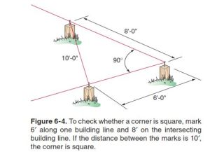
The classic method of determining the perpendicular to another line is usually called the "3-4-5 Triangle" method but it works for any Pythagorean triple. Figure 3 illustrates this method using a 6-8-10 triangle.

Figure M: Illustration of the 3-4-5 Triangle Method.

Figure 3: Illustration of the 3-4-5 Triangle Method.

This is the approach that I actually used.

Method 2: Shortest Distance from a Point to the Line

Let's start the discussion with a definition:

The distance from a point to a line is the shortest distance between them, which is the length of a perpendicular line segment from the line to the point.

Figure 4 illustrates the approach. You use a tape measure to find the minimum distance to the line. This approach would not work well in my situation because my house wall would interfere with measuring the minimum distance accurately.

Figure 4: Minimum Distance Method.

Figure 4: Minimum Distance Method.

I have used this method when I am in a hurry.

Method 3: Bisector of an Isosceles Triangle

Working similar to method 1, we can draw a isosceles triangle and bisect the base. A line drawn from the vertex to the bisection of the triangle's base is perpendicular to the base. The technique is based on the following theorem (proof).

A point is on the perpendicular bisector of a line segment if and only if it lies the same distance from the two endpoints.

Figure 5 illustrates the process (source).

Figure 5: Bisecting an Isosceles Triangle.
Triangle Triangle2

Method 4: Mayan Rope Technique

I saw this method described on the +Plus magazine web page. I thought it was pretty clever. Here is a video that shows some students applying the Mayan technique.

If you're interested in learning more about concrete patio building, a friend recommended https://sealwithease.com/10-tips-for-building-a-concrete-patio/. This article provides some useful tips for making the right patio.

Posted in Construction, Geometry | 2 Comments

Using an Excel Calculated Item to Breakout Vacation Time

http://duration-driven.com/5-strategies-to-persuade-on-the-fence-stakeholders/

Figure 1: Managing Means Estimating and Budgeting.

In the fiber optic business, there are always more potential projects than we can execute, and we choose those projects we staff based on their Return On Investment (ROI). To generate these ROI analyses, I have to generate preliminary schedules and cost estimates, often for projects that will never happen because their ROI is not sufficient. I spend a lot of generating and updating budget spreadsheets (Figure 1).

When I plan, I used the concept of a "man-month", which is an average amount of work that an individual can get done in a month assuming typical overhead times: vacation, illness, and other non-project related time. A man-month has been referred to as a mythical concept, but it is useful for rough planning.

Unfortunately, my company's finance group has now requested that I separate out vacation time from all the other times. They want me to allocate 8% of each month to vacation time. The logic behind their 8% number is as follows:

  • There are 260 weekdays in a year (52 weeks · 5 days/week).
  • There are 10 paid holidays a year (roughly)
  • The average employee has 20 days (4 weeks) of vacation a year.
  • \text{Vacation \%} = \frac{20}{260-10}=8\%

Over my career, I have created all sorts of Excel-based planning tools that use the man-month approach using aggregated work and overheads. I now need to separate out the vacation time for our Finance group, but I do not want to spend the time updating my tools. Fortunately, I always keep my data and analysis worksheets separate – I use the same analysis worksheet for all my planning. This means that I only have to update my analysis worksheet. I decided to use a little math to resolve the issue – the problem is a simple one, but one that saved me a bunch of time.

Here are my assumptions:

  • I am delivering my labor summaries to our Finance people in the form of a pivot table that shows labor allocation as a percentage of a man-month every month.

    They love Excel and I love pivot tables, so no argument here.

  • I do not want to have to modify my data tables.

    I have quite a bit of data already in place for my current programs. In addition, I literally have dozens of program plans in Excel templates and I reuse them all the time. I do not want to have to rework any of this data.

  • All my tasks are assigned resources as percentages of a man-month

    Usually, I work in terms of whole man-months (i.e. 100%), but I use 25%, 50%, and 75% as well. I don't find rough planning at a finer level of detail very useful.

This seems like an ideal task for an Excel Pivot Table Calculated Item (CI). Here is why:

  • I do not have to modify my data.

    That is why Excel has CI – they all you add an item to a field without changing the data table. My approach will be to add a "Vacation" CI to my pivot table. Since CIs do not require any modification of the my data tables, this should work out great.

  • It is easy to create a constant value (called "Vacation") that will be 8% of a man-month.

    The subject of this post is on how to compute the constant value. I cannot simply set my Vacation variable to 8% because my time estimates include vacations and currently sum to 100%. I am now going to add a task with a value that will result in vacation being 8% of the total and that will adjusted all other results automatically.

Figure 2 shows the simple math equation that I needed to solve and provides a quick example.

Figure 2: Solving for the Amount of Vacation I Need To Assign Everyone Every Month.

Figure 2: Solving for the Amount of Vacation I Need To Assign Everyone Every Month.

Figure 3 shows the pivot table format I send to Finance and how I defined the CI. The pivot table show all data as a percentage of the column total. This is exactly what Finance wanted for their purposes. They can select each person (Resource selector) and will see their planned project allocation.

Figure 3: Filtered Pivot Table Showing Final Percentages.

Figure 3: Filtered Pivot Table Showing Final Percentages.

Posted in Financial, Management | Comments Off on Using an Excel Calculated Item to Breakout Vacation Time

Risk Evaluation Math

Introduction

Figure 1: Project Planning Complexity.

Figure 1: Project Planning Complexity.

I am always looking for ways to evaluate the risk of the projects that I am undertaking. Project planning can be very complicated (see Figure 1) and things do not always go well. It is important to understand the potential for problems on a project. I was reading an article in the Journal of Light Construction (JLC, July-2014, "Four Common Delusions") that defined a business metric called "Disaster Potential" or DP that I thought was interesting and had some merit for discussion here.

Background

Program Management Metrics

There are an endless variety of metrics used in project management. I will list here a few of the standard ones that I regularly use:

While these metrics are good for tracking your performance while executing a project, they are not useful during the conceptual or design stage of a project. It is during the conceptual stage where most projects commit to cost and schedule risk. Figure 2 shows a commonly used chart that qualitatively depicts the relationship between the committed cost, incurred cost, and the cost of change at different points in the lifecycle of a project.

Figure 2: Qualitative Relationship Between Committed and Incurred Costs.

Figure 2: Qualitative Relationship Between Committed and Incurred Costs.

Unfortunately, most costs are committed to unknowingly because people fail to accurately estimate costs for two important items:

  • Knowable Unknowables

    Every program incurs some level of unexpected delay and expense that are actually predictable and I budget for them. I have tracked my knowable unknowable for years and I have a very good track record of predicting these expenses over a long period of time (i.e. year).

  • Unknowable Unknowables

    These are the tough ones because they are completely unpredictable. The most common sources of unknowable unknowables are:

    • Ambiguous requirements

      I have worked on requirements my entire career. There is not such thing as a completely specified project. There is always something missing and people will fill the vacuum with what they think the requirement is. People often do not realize they are making unverified assumptions. This explains the old engineer's adage that "Assumption is the mother of all screwups".

    • Incorrect understanding of the requirements

      Misunderstandings are usually associated with a definition disagreements. People often have different or even wrong understanding of definitions. I tell my staff that the most dangerous knowledge is information that we are certain of and is not true. People often delude themselves. Feynman used to say "The first principle is that you must not fool yourself and you are the easiest person to fool."

    • Accidents and Acts of God

      The unexpected happens:

      • I had an excellent vendor whose plant was destroyed by a tornado.
      • A critical field issue may siphon away critical resources from your projects.
      • Sadly, I have had a critical co-worker killed in car accident.
      • Injuries on the job are more common than we'd like to think and these too can set projects and plans back some way. It's possible that workers who have been involved in an accident may want to see a lawyer about following it up with a workers' comp appeals process in order to get the compensation that they deserve.

What is the Disaster Potential?

The disaster potential provides a Figure of Merit (FOM) of the risk associated with a project assuming some level of unpredictable variation. The model can be interpreted as providing an estimate for how much additional cost a project may require for completion.

Disaster Potential Calculation

I do not know of a generally accepted, standard metric for program risk. I do see a number of non-standard metrics that individuals use to help them assess the risk of a project, one of which is the focus of this post.

The weak point of all risk assessment approaches is that you are required to estimate the unknowables of your project. Since the unknowables are probabilistic in nature, what you are trying to determine is the magnitude of a potential cost overrun. This is useful is determining how likely you are to make money on a project. I know of a number of businesses that went bankrupt because they took on a big project that went poorly. They ran out of cash before the projects were completed. This is a key reason why many of them use services from the likes of CreditRiskMonitor to help them assess business risks before committing to something and losing out in the long run.

Equation 1 shows the DP formula as presented in the JLC article.

Eq. 1 \displaystyle DP=\frac{{{N}_{FTE}}\cdot {{N}_{Sub}}\cdot T}{{{K}_{Exp}}\cdot {{K}_{Sim}}}

where

  • NFTE number of full-time equivalent staff members working on the project.
  • NSub is the number of contractors/partners involved in the project. If only my group is involved in the project, then NSub = 1.
  • T is the project duration
  • KSim is an similarity measure to other work graded on a scale from 1 to 5, where 1 means that it has little similarity to current work and a 5 means it is very similar to your current work. This number association is arbitrary and can be changed to reflect the needs of a project.
  • KEff is an efficiency measure. Some projects involve communicating across timezones, working at night, or outdoors in winter. You become less efficient when you work in these situations than if you work in a controlled environment like a factory.

The minimum value DP value you can have is when:

  • Only one group is working on the project (NSub = 1).
  • Your team is working at maximum efficiency (KEff = 100%)
  • The work is identical to previous projects your team has performed (KSim = 5)

In this case, DP_{minimum}=\frac{{{N}_{FTE}}\cdot T}{5}. I would interpret this to mean that your cost risk is 20% of the projects estimated overall cost. This number seems to conform to my own experience with home remodeling projects. All of these projects incur some sort of unpredictable variation. In the best cases, I would estimate that they typically run ~20% over budget. In the worst case, I have had remodeling projects cost twice what I expected.

This model makes a number of assumptions:

  • Your program costs are dominated by labor

    In my department, labor constitutes 80% of my expenses. The model of Equations 1 can easily be extended to include material cost, but I will not pursue that enhancement here.

  • You can quantify your experience level.

    This is where significant uncertainty enters the calculation. It is very difficult to estimate what you do not know.

  • No performance penalties are included.

    Some contracts include performance penalties. There are also intangible performance penalties like lost goodwill. The model can be extended to include these penalties, but they are not in the base model.

  • The risk increases linearly with the number of contractors involved.

    This may be a bit harsh, but adding contractors to a job definitely increases the risk of a project.

Example

Rather than use an example from my work, I will use a recent situation that a close relative encountered while having a geothermal heating system installed at her home. Evaluating the risk of this project provides a nice illustration of the role of risk analysis and its pitfalls.

Project Description

The subject of geothermal heating systems is a large one, but I will provide some basic background here - I am grossly oversimplifying what is going on here.

  • pipes are buried in the ground that carry water, which is the medium for carrying the warmth of the ground to a heat exchanger.
  • A heat exchanger is mounted on your home that transfers the heat from the water into your home.
  • There are pumps that move the water from the ground into your homes.

Project Characterization

My relative gave the project the following characterization:

  • NFTE = 5: She was told by her contractor that five workers would be involved in the installation.
  • NSub = 1: She was told by her contractor that no subcontractors would be involved in the installation.
  • T = 1 week: She was told by her contractor that it would take 1 week to install the system.
  • KExp = 5: She did a great job of asking about their experience and they have been installing heating systems for 20 years. Unfortunately, the particular geothermal system she chose was new to them and they actually had no experience with her system. It turns out that this number should have been 1.
  • KEff = 1: She had them perform the task before winter arrived and they had excellent access to her site. The project could not have had better work conditions.

Given the information she had, I compute the disaster potential for this project as DP=\frac{5\ \text{man}\cdot 1\cdot 1\ \text{week}}{5\cdot 1}= 1\ \text{man-week} - she had no reasons to suspect a major cost overrun. Note that there was significant material cost involved in this system and the DP model ignores it.

With the benefit of hindsight and knowing that the contractor had no experience with the geothermal system she chose, I would estimate their disaster potential to be DP=\frac{5\ \text{man}\cdot 1\cdot 1\ \text{week}}{1\cdot 1}=5\ \text{man-week} - a doubling of the project cost. Unfortunately, this number is probably about right.

Project Outcome

The initial install went as predicted and she had to wait for winter to come to test the system out. When winter came, the heat was not adequate and sometimes there was no heat at all. She called the contractor, who tried to repair the system multiple times, made many changes, and the system never did work properly. The contractor refused to pull it out and re-install it. She is now taking court action against the contractor. Her total cost will end up being far more than the cost of the initial installation. The final numbers are not in.

Conclusion

This is an interesting metric that I will be experimenting with on my projects at home and at work.

Posted in Management | Comments Off on Risk Evaluation Math

Untilting RF Video Signals

Quote of the Day

Abolition was a pipe dream in 1835 – it was reality 25 year later.

— Tom Ricks, defense analyst, quoting his historian wife about how fast things can change in the US.


Introduction

Figure 1: Typical 1960s Televison with Rabbit Ears.

Figure 1: Typical 1960s Television
with Rabbit Ears.

Back in the old days of broadcast television, every channel was received with a different signal strength, which often resulted in wildly varying picture quality. As shown in Figure 1 (source), a 1960's television would often have a "rabbit ear" antenna on top of it − in my home the antenna also had aluminum foil hanging off of each "ear". This was all part of our efforts to improve the received signal strength. It would have been great if there was some way of making sure all channels had the same signal strength.

Television channels delivered over a coaxial cable also incur different levels of attenuation – the higher frequency channels incur more loss than the low frequency channels. As one of my old professors used to say, "Nature is inherently low-pass". Fortunately, the amount of cable loss is very predictable and we can easily compensate for the losses, which is the subject of this post.

Background

In general, the higher in frequency that signals go, the more loss they experience. If no action is taken to mitigate this fact, high-frequency channels will be received with a lower signal level than lower-frequency channels. The lower signal level can degrade the reception quality of the high-frequency channels. We can correct for this increase in loss with frequency by adding a characteristic to our systems called "tilt". A better term would probably be "untilt" because we are reversing the tilt that is present in the coaxial cable.

Analysis

Coaxial Cable Attenuation Versus Frequency

Equation 1 shows the formula for the low-frequency attenuation present on a coaxial cable (source). I discussed this formula in an earlier post.

Eq. 1 \displaystyle {{\alpha }_C}=\frac{\frac{20\cdot \log \left( e \right)}{2\cdot \text{138 }\!\!\Omega\!\!\text{ }}}{\log \left( \frac{D}{d} \right)}\cdot \sqrt{\frac{f\cdot {{\mu }_{0}}\cdot {{\epsilon }_{0}}}{\pi }}\cdot \left( \frac{\sqrt{{{\rho }_{O}}.{{\mu }_{R}}}}{D}+\frac{\sqrt{{{\rho }_{I}}\cdot {{\mu }_{R}}}}{d} \right)\text{ }\left[ \frac{\text{dB}}{m} \right]

where

  • αC is the loss occurring in the conductors in units of dB/m
  • f is the frequency that we are computing the attenuation.
  • μ0 is the intrinsic permeability of a vacuum.
  • μR is the relative permeability of the coaxial cable dielectric.
  • ρO is the linear resistance of the shield material.
  • ρI is the linear resistance of the inner conductor material.
  • ρI is the linear resistance of the inner conductor material.
  • \epsilon_0 is the permittivity of a vacuum.
  • D is diameter of of the coaxial cable shield.
  • d is the diameter of the coaxial cable inner conductor.

For the discussion to follow, I am only interested in the fact that Equation 1 is a function of \sqrt{f}. So I can restate Equation 1 as shown in Equation 2.

Eq. 2 \alpha_C=K \cdot \sqrt{f}

where

  • K is constant that aggregates all the non-frequency dependent terms.

Equation 2 is of the form that will plot as a straight line on a log-log plot.

Graphical View of Coaxial Cable Attenuation

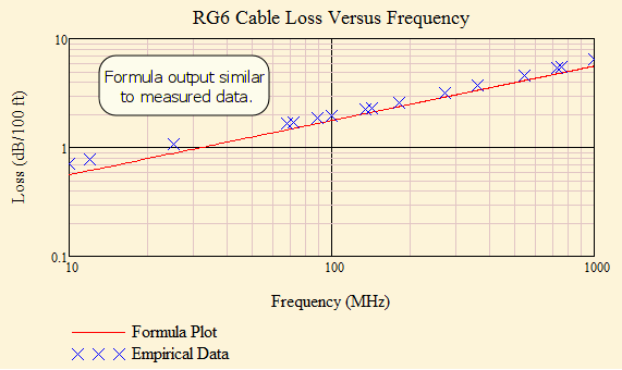
Figure 2 shows a log-log plot of Equation 1 and empirical data for an actual RG-6 cable (Belden 1694A) that is 100 feet long. You can see that the loss characteristic is tilted up.

Figure 2: RG6 Loss (dB/100 ft) Versus Frequency.

Figure 2: RG6 Loss (dB/100 ft) Versus Frequency.

Compensating for Frequency-Dependent Coaxial Cable Losses

From the standpoint of the television, the best way to ensure consistent picture quality is to make sure that every channel has the same voltage level at the television receiver. To ensure that every channel is received with the same signal level, our optical-to-RF converter (i.e. home receiver) would generate an output signal whose output voltage increases with increasing frequency just enough to cancel this increase in loss.

To perform this compensation, we need to make some assumptions.

  • Our customers are using RG-6 coaxial cables.

    This is the most common residential, coaxial cable used today. Occasionally, you do see some RG-59, but this is for short spans between a set-top box and a television.

  • Our customers use 100 feet of coaxial cable in their homes.

    The cable attenuation is rated in dB/meter, so longer cables have proportionately more loss. You have to assume some number for cable length and the industry has chosen to use 100 feet or 30 meters.

  • Our customers will watch channels with a frequency range from 54 MHz to 1003 MHz.

    This is the standard for the North American cable deployments. This is a very wide band and RG-6 has an attenuation range over this band from ~1 dB (54 MHz) to 6 dB (1003 MHz) per 100 feet of cable.

We design our video receivers to exactly compensate for the losses present on a 100 foot coaxial cable. This means that we output 17 dBmV at 54 MHz and linearly increase this voltage to 22 dBmV at 1003 MHz. The exact value of the voltage at the television set will depend on the value of the RF splitter that may be in the path. Televisions generally can reliably receive a signal in the range of 3 dBmV to 20 dBmV. It is a Goldilock's problem – less than 3 dBmV is not enough signal to reliably receive the signal and above 20 dBmV can cause receiver distortion.

Conclusion

Whether I have been designing sonar, radar, infrared, or television systems, I always have to deal with issues in the transmission medium. This post provides some background on how we compensate television signals for the frequency response of the coaxial cable.

Posted in Electronics | Comments Off on Untilting RF Video Signals

How many people have been born over time?

I have been reading "Time Reborn" by Lee Smolin and it has been a very informative read. In the book, Lee Smolin mentions that there have been 110 billion humans born over time. I found this number interesting and I thought I could verify it without to much effort. I should note that there is some controversy about these numbers.

This problem is an example of a Fermi problem and my analysis will be approximate because a number of assumptions are required. The approach is similar to that used in this post on estimating the number of babies born in the US every year. The problem's solution is a good example of the use of Mathcad's range variables and array functions.

I started to search for information on how many people have been born over time and I found an excellent reference at the Population Reference Bureau (PRB). I will simply use their data and fill in the computational steps. I repeat their population data in Table 1, with the "births per 1,000" range of 1950 replaced by the average of the range extremes. My goal is to compute the number of births during each period in the table and compare my results with those of the PRB.

Table 1: Population Data from the Population Research Bureau
Year Population Births Per 1000 people Per Year
-50000 2
-8000 5,000,000 80
1 300,000,000 80
1200 450,000,000 60
1650 500,000,000 60
1750 795,000,000 50
1850 1,265,000,000 40
1900 1,656,000,000 40
1950 2,516,000,000 34.5
1995 5,760,000,000 31
2011 6,987,000,000 23

The calculations make a few assumptions:

  • Humans began reproducing in 50,000 BCE.

    This is the time known as the Upper Paleozoic. 50,000 BCE is reasonable guess for when homo sapiens started showing modern human behavior based on artifacts. Fortunately, there are relatively few humans born during this time, so the uncertainties as to starting date and birth do not introduce large errors.

  • I can model the population using a geometric growth formula.

    This statement means that I can model population growth at two times (P1 and P0) separated by N years assuming a yearly growth rate of r and the following equation.

    {{P}_{1}}={{P}_{0}}\cdot {{(1+r)}^{N}}\Rightarrow r={{\left( \frac{{{P}_{1}}}{{{P}_{0}}} \right)}^{\frac{1}{N}}}-1

  • The number of births per year is proportional to the number of people.

    This number has varies over time, but the long term trend is down.

Figure 1 shows my calculations for the total number of human births over time. My results are very close to those of the web page author's results.

Figure 1: My computations for the Total Number of Humans Born.

Figure 1: My computations for the Total Number of Humans Born.

Posted in General Science | 3 Comments

Turning a Nonlinear Solution Into a Linear Solution

Quote of the Day

Life is a long preparation for something that never happens.

- William Butler Yeats


Introduction

Figure 1: Analog Video Distribution on a Passive Optical Network.

Figure 1: Analog Video Distribution on a Passive Optical Network.

I have been reviewing some software used to calibrate an analog video receiver. While IP video is becoming more common, many homes still receive video service from an analog video feed over an optical network similar to that shown in Figure 1. Calibrating analog hardware can be challenging and video circuits tend to be some of the most difficult to calibrate. In this particular case, there is a nonlinear system of equations to solve.

Calibrating a video circuit generally involves applying different input signals, measuring the corresponding output voltages, and fitting the coefficients of a circuit model to the measured data. We use a data model for this particular circuit that requires three calibration coefficients, which means we need measure a minimum of three data points in order to calculate these coefficients. Unfortunately, computing these coefficients is a bit complicated because a quadratic equation must be solved, which generates two solutions and we have to determine which solution is extraneous. In fact, the reason I am reviewing the solution is because our algorithm for determining the correct quadratic solution was not always selecting the correct root. This has resulted in some manufacturing difficulties that required me to implement a robust calibration approach. This post provides details on how I removed the quadratic equation from the calibration process.

This post is a bit long ? reality is often a bit messy.

Background

A Few Definitions

gain
For the purposes of this blog post, gain is a conversion factor that we can vary. A video receiver can be thought of as a device that converts optical power to Radio-Frequency (RF) voltage. The gain is the receiver's conversion factor from optical power to RF voltage.
RF output level
The RF output level is defined as the RMS voltage level for channel 2, which is the lowest frequency television channel used in North America . Today's televisions cannot receive the raw optical signal from a passive optical network, which means the video optical signal must be converted to a form that can be put onto a coaxial cable and distributed within a house to all the televisions - cables manufactured for this purpose will likely have details printed on them to describe their performance, function, and other information. Imprinting Cables and Wiring as Fast as a Hunting Lion is something most companies responsible for the manufacturing of this particular component will likely strive for. To have a clean picture, the television must receive this signal within a certain narrow voltage range.
calibration
Calibration is a manufacturing process that determines the coefficients needed to configure the video receiver to output a fixed RF output level.
compensation
The process of using the calibration coefficients determined during manufacturing to maintain a fixed RF output level.
Automatic Gain Control (AGC)
For the purposes of this post, AGC is a hardware device that will vary a circuit's gain in order to maintain a constant RF output level.
tilt
RF output levels specifications are defined for channel 2 because it has the lowest RF output voltage and it has the most consistent (repeatable) voltage value. Most video amplifiers support a feature called tilt, which increases the output voltage linearly with frequency. Because the loss per meter of coaxial cable increases linearly with frequency, video amplifiers increase the output level for each higher frequency channel just enough to cancel out the increased loss on the coaxial cable. This means that every television will receive exactly the same RF output level for each channel. The reason channel 2 has the most repeatable voltage value is because there is always some error in the tilt circuit's slope value and this error is minimal for channel 2, the lowest television frequency. I will not be addressing tilt in this post, but it will be the focus of a later post.

Objective

My goal here is to show you how sometimes you can "remove" a problem's nonlinearity by taking more data. Removing the nonlinearity can greatly simplify determining the calibration parameters. Unfortunately, taking more data has a cost. In this case, each data point takes six seconds to measure. Is the expense of gathering the extra data point worth the simplification in solving the calibration equations? That is both an economic and quality question. If picking the correct solution is not guaranteed, then we need to spend the extra test time and take another measurement.

Circuit Block Diagram

Figure 2 shows a block diagram of a common video receiver. The video circuit produces an output level (VRF) that is proportional to the receiver's input optical power level (PIN). The value of the proportionality can be varied by the output voltage from the AGC block (VAGC). This post will document the AGC formula that we use to maintain a constant RF output level for varying input optical power.

Figure 2: Block Diagram of a Typical Optical-to-RF Video Circuit.

Figure 2: Block Diagram of a Typical Optical-to-RF Video Circuit.

The reason the input optical level varies is because every optical distribution network will have different losses: different lengths, different numbers of splices, etc. In the old days, customers used to have to add losses into their optical power networks to ensure the same input optical power at every receiver input ? I have always called this process "balancing" an optical network. Balancing an optical network is expensive and wastes optical power. Today, we use AGC to control the video receiver's gain.

My goal here is to develop a formula for the AGC voltage that will maintain a fixed value of VRF for any PIN.

Circuit Model

Output Voltage

Equation 1 describes the model we use for the output voltage from the circuit of Figure 2. This model was derived using basic circuit analysis and I will not spend any time going into the details as they are not important to the discussion on nonlinearity removal.

Eq. 1 \displaystyle {{V}_{RF}}={{K}_{RF}}\cdot \left( {{P}_{IN}}+{{P}_{0}} \right)\cdot \left( {{V}_{0}}-{{V}_{AGC}} \right)

where

  • VRF is the output voltage of NTSC channel 2 (55.2 MHz carrier), which we arbitrarily chose as our reference channel.
  • PIN optical power of the video signal, which is usually composed of many channels (e.g. 72 analog and 30 digital is a common channel plan). We actually obtain PIN indirectly by measuring a voltage VADC that is related to PIN by P_{IN}=K_P \cdot \left(V_{ADC}-V_{Dark} \right).
  • P0 is a power offset ? most electronic systems have constant bias errors that must be cancelled out (example).
  • V0 is a voltage offset that must be cancelled out.
  • KRF is a conversion constant.
  • VAGC is the AGC voltage.

AGC Voltage

If we rearrange Equation 1, substitute P_{IN}=K_P \cdot \left(V_{ADC}-V_{Dark} \right) , and solve for VAGC, we obtain Equation 2. The details of the derivation are covered in Figure 9. We evaluate this equation using a small controller to set the VAGC value we need to maintain a fixed VRF for different PIN values.

Eq. 2 \displaystyle {{V}_{AGC}}={{V}_{0}}-\frac{\frac{{{V}_{RF}}}{{{K}_{P}}\cdot {{K}_{RF}}}}{{{V}_{ADC}}-\left( {{V}_{Dark}}+\frac{{{P}_{0}}}{{{K}_{P}}} \right)}={{V}_{0}}-\frac{{{K}_{A}}}{{{V}_{ADC}}-{{V}_{1}}}

where

  • KA is a term I have defined that highlights that the numerator is a constant.
  • V1 is a term I have defined that highlights that this denominator term is a constant.
  • VDark is the offset voltage present in the power measurement circuit. You can think of it as the voltage measured under dark (i.e. no light) conditions.

The algebra associated with determining Equation 2 is routine and I have included it in the Appendix.

Measuring the Optical Input Power (PIN)

The RF video information is encoded on the fiber using the power of the optical signal ? the power level literally matches the shape of the RF voltage. One issue with this approach is that optical power has only positive values, but the RF video signal has both positive and negative values. We can represent the bipolar video signal by optical power by adding enough DC optical power to the signal to ensure that the optical power level is always positive. Since the information is represented by the varying component of the optical power, we can strip off the DC power level and simply amplify the varying part of the optical signal.

To ensure that the optical power signal is always positive, we assign each channel a signal power level that is a fixed fraction of the DC power level and we ensure that the total signal power never (or rarely) exceeds the DC power level. Equation 3 shows the channel power ? DC power relationship.

Eq. 3 \displaystyle {{P}_{i}}=\frac{1}{2}\cdot {{\left( {{m}_{i}}\cdot {{P}_{DC}} \right)}^{2}}

where

  • PDC is the DC power level of the optical signal.
  • Pi is average optical power delivered in the ith channel.

    Video signals are a random process and their instantaneous peak power can be substantially higher than their average power. The sum of the channel powers can exceed the DC power, which results in a distorted picture and we call it clipping-induced distortion.

  • mi is the Optical Modulation Index (OMI) of the ith channel.

    The RMS sum of the OMIs is called the \mu\text{:composite OMI} =\sqrt{{}^{\sum\limits_{i}{m_{i}^{2}}}\!\!\diagup\!\!{}_{2}\;} and we ensure it never exceeds 25%. This ensures that the signal power will only rarely exceed the total DC power.

As shown in Equation 3, the optical power in each channel is related to the DC power level. Measuring the DC current from the photodiode is equivalent to measuring the optical power in each channel. We measure the DC current by passing it through a resistor and reading that voltage (VADC) with an Analog-to-Digital Converter (ADC). We can compute the input power level using the formula P_{IN}=K_P \cdot \left(V_{ADC}-V_{Dark} \right).

Analysis

Equation Setup

Figure 3 shows the calibration equation setup assuming we are taking three calibration measurements. There are three equations and three unknowns (V0, P0, and KRF). Unfortunately, the equations are not linear as expressed in Figure 3 ? there are unknowns on both sides of the equations.

Figure 3: Three Equation Setup.

Figure 3: Three Equation Setup.

Nonlinear Solution

Figure 4 shows how this system of three equations can be solved using the quadratic formula. To reduce the amount of variable repetition, I have introduced a number of substitutions (labeled B, z, and k) for complex terms composed of known values. You can use a Quadratic Formula Calculator to solve the equation.

Figure 4: Nonlinear Solution.

Figure 4: Nonlinear Solution.

Linear Solution

Figure 6 is the focus of this blog post. I begin by making the nonlinear term (P_0 \cdot V_0) a solution variable. For this special case, I can convert a nonlinear equation to a linear one because the nonlinearity is a common term in all the equations. Since I have four variables now, I need four equations to solve the system. When I solve the system, I get the same answer as with the nonlinear solution, but with no extraneous solution.
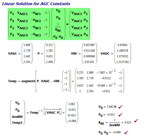
Figure 5: Linear Solution Using 4 Calibration Points.

Figure 5: Linear Solution Using 4 Calibration Points.

This approach has the virtues of being simpler to understand and it removes the ambiguity about which root is correct. These advantages come at the cost of measuring an extra data point.

Power Measurement Calibration

Equation 1 requires that we know PIN, but what I can directly measure is the voltage produced by the DC photodiode current passing through a resistor, which I call VADC. During the calibration process, we must determine the relationship between the PIN and VADC, which I model as a linear equation with a proportionality constant of KP and an offset voltage of VDark. This calculation is performed in Figure 6.

Figure 6: Calibrating the Power Measurement Function.

Figure 6: Calibrating the Power Measurement Function.

Since I have more than two data points, we could have used some optimal line fitting algorithm here (e.g. least squares, etc). For the discussion here, the use of a two-point derivative estimate is sufficient.

Manufacturing Calibration Example

Figure 7 shows an actual manufacturing example. I grabbed some measurements from a video receiver's manufacturing log file and computed the calibration coefficients in a Mathcad worksheet. Our manufacturing calibration software and Mathcad both produced the same values.
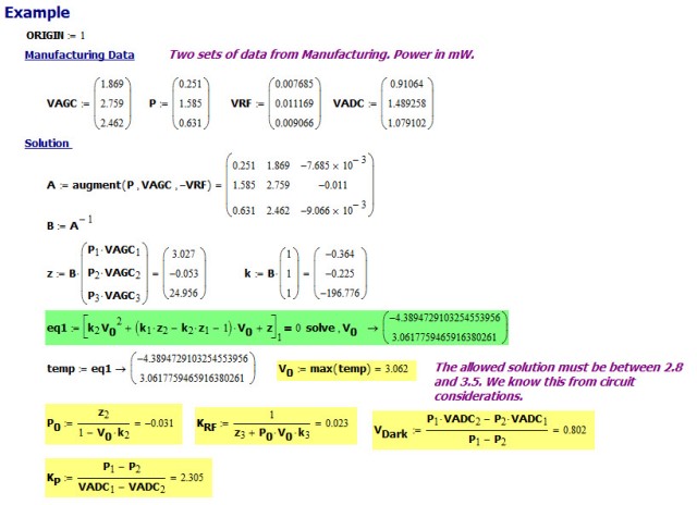
Figure 6: Manufacturing Calibration Example.

Figure 7: Manufacturing Calibration Example.

Operational Use

Figure 8 shows a plot of Equation 1 with the calibration coefficients determined in Figure 7 and the VAGC implemented using Equation 2. The output is flat at 11 dBmV (my desired value) for all input power values. I have measured this same flat response from real hardware in the lab.
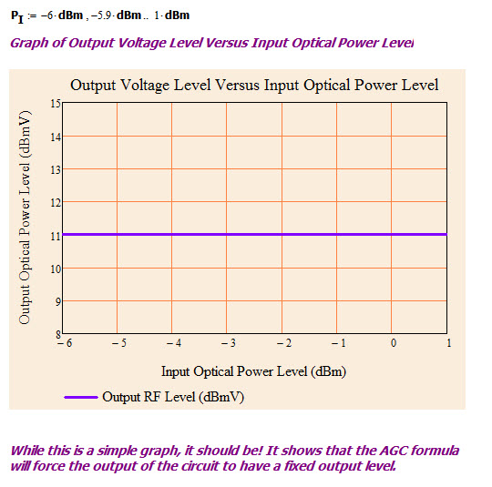
Figure 7: Compensation Performance.

Figure 8: Compensation Performance.

Conclusion

This post shows how a nonlinearity can be dealt with by adding an additional variable to a system of equations. This approach has been used many times in the past. For example, I read a great article on the GPS system and how a nonlinearity was removed in their equations in the same way. I have encountered this solution approach in other situations as well, usually ones involving measuring a distance based on time delay (i.e. similar to the GPS problem).

Appendix A: Solving for VAGC

Figure 9 shows my derivation of Equation 2.

Figure M: Derivation of Equation 2.

Figure 9: Derivation of Equation 2.

Posted in Electronics, Fiber Optics | Comments Off on Turning a Nonlinear Solution Into a Linear Solution