It's Warm Out and the PVC is Getting Longer ...

Quote of the Day

Far better an approximate answer to the right question, which is often vague, than an exact answer to the wrong question, which can always be made precise.

— John Tukey


Introduction

I live in Minnesota -- where winter temperatures can be as low as -36 °C (-33 °F) and summer temperatures can be as hot as 38 °C (100 °F). Because most things expand when our days get hotter, we occasionally have things like doors and windows that are too tight in the summer and too loose in the winter. Today, I encountered a PVC pipe that was installed during the heat of last summer and it had ripped itself free of its mounting brackets during the cold of winter. Of course, it is summer now and the pipe is back to its installed length. I was asked by an electrical equipment installer today how much length variation should he plan for when using PVC pipe outdoors. It turns out the National Electrical Code (NEC) actually has a table that addresses this question and I will discuss in this post how that table was generated. Let's discuss the answer I gave this installer.

Background

PVC Expansion Table from the NEC

I referred the electrical installer to Table 1, which is from the NEC.

Table 1: NEC Table 352.44 Expansion Characteristics of PVC Rigid Nonmetallic Conduit
Temperature Change (°C) Length Change of PVC Conduit (mm/m) Temperature Change (°F) Length Change of PVC Conduit (min/100 ft) Temperature Change (°F) Length Change of PVC Conduit (min/100 ft)
5 0.30 5.00 0.20 105 4.26
10 0.61 10.00 0.41 110 4.46
15 0.91 15.00 0.61 115 4.66
20 1.22 20.00 0.81 120 4.87
25 1.52 25.00 1.01 125 5.07
30 1.83 30.00 1.22 130 5.27
35 2.13 35.00 1.42 135 5.48
40 2.43 40.00 1.62 140 5.68
45 2.74 45.00 1.83 145 5.88
50 3.04 50.00 2.03 150 6.08
55 3.35 55.00 2.23 155 6.29
60 3.65 60.00 2.43 160 6.49
65 3.95 65.00 2.64 165 6.69
70 4.26 70.00 2.84 170 6.9
75 4.56 75.00 3.04 175 7.1
80 4.87 80.00 3.24 180 7.3
85 5.17 85.00 3.45 185 7.5
90 5.48 90.00 3.65 190 7.71
95 5.78 95.00 3.85 195 7.91
100 6.08 100.00 4.06 200 8.11

Linear Expansion Formula

Equation 1 shows a commonly used formula for thermal expansion. This is the formula that was used by the NEC people to generate Table 1. They assumed that for PVC \alpha =60.84{}^{\mu m}\!\!\diagup\!\!{}_{m\cdot {}^\circ C}\;. For comparison, steel has an expansion coefficient of 13 µm/(m·°C).

Eq. 1 \displaystyle \Delta L\left( \Delta T,L \right)=\alpha \cdot L\cdot \Delta T

where

  • ΔL is change in length with temperature.
  • ΔT is the change in temperature from the reference temperature.
  • α is the temperature coefficient of thermal expansion.
  • L is the length of the object at the reference temperature.

    I usually base my estimates on the temperature at the time of install. Since most of our products are installed in the heat of the summer, any PVC pipe used does not get too much longer but will get a lot shorter when winter comes.

Analysis

Exact Calculation

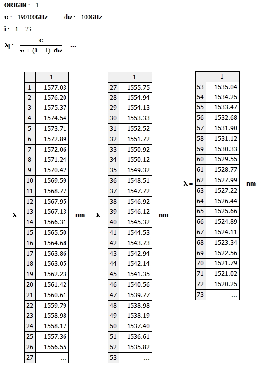
Figure 1 shows my calculations that duplicate part of the NEC table. The rest of the table is done similarly. As you can see, the calculations are a straightforward implementation of Equation 1.

Figure 1: NEC Table Generated By Mathcad.

Figure 1: NEC Table Generated By Mathcad.

Rule of Thumb

I generally do NOT use Equation 1 when I need to estimate the amount of PVC expansion. Because I live in the US, the installers uses inches and °F for length and temperature units, respectively. Using Table 1, notice that 100 feet of PVC changes in length about 4 inches (equals 1 inch over 25 feet of length) over a 100 °F temperature range. Since the thermal expansion formula (Eq. 1) is linear with respect to temperature difference and length, I can write down Equation 2 directly.

Eq. 2 \displaystyle \Delta L\left( \Delta T,L \right)=1\text{ in}\cdot \frac{L\left[ \text{feet} \right]}{25\text{ ft}}\cdot \frac{\Delta T}{100\text{ }\!\!{}^\circ\!\!\text{ F}}

Most of the time, I can approximate this equation in my head by assuming that the length of PVC pipe changes by ~1 inch for every 25 feet of length over a 100 °F temperature change. This rule of thumb is close enough for most of my work.

Conclusion

I frequently encounter problems caused by people failing to account for the changes in material dimensions with temperature (e.g. frost heave). I must admit that I also have forgotten to account for expansion and contraction with temperature with my personal projects. My goal in this post was to show how a rule of thumb for PVC can be developed that is good enough for use in most cases. This process is similar to how other rules of thumb are developed.

The same type of calculations can also explain why vinyl siding (made primarily of PVC) moves so much between winter and summer. For some supporting evidence of my rule of thumb, here is a quote from a home inspection web site on the expansion of vinyl siding.

A 12-foot length will vary in length up to 1/2 inch over a 100°F temperature change.

This statement is similar in form to my Equation 2.

Posted in Construction, General Science | 2 Comments

Maximum Phone Line Length Math

Quote of the Day

All right, sweethearts, what are you waiting for? Breakfast in bed? Another glorious day in the Corps! A day in the Marine Corps is like a day on the farm. Every meal's a banquet! Every paycheck a fortune! Every formation a parade! I LOVE the Corps!

— Sergeant Apone in the movie "Aliens". I love this line.


Introduction

I was asked today how long a telephone line in North America can be and still work properly. This is an interesting question and worth writing about here. The US still has about 112 million of these lines in service (2011), however the number of lines is declining each year. I can see the days of the classic copper phone line coming to an end over the next few decades. Like analog video, it will eventually be replaced by digital services. For a fiber optic deployment (i.e. no copper), the old phones lines can re-purposed to carry the power needed by the fiber optic interface if AC power is not available. To carry power, the resistance of the line -- which is determined by the length and cross-sectional area of the line -- becomes very important. When carrying voice signals, phone line resistance was limited to ensure that the central office could detect the phone going off-hook. This post will use the maximum allowed line resistance to determine the maximum possible line length.

The answer to the maximum length question is "it depends" -- which is the answer to all interesting engineering questions. It depends on things like:

  • the telephone standards the line was built to (e.g. TR-57 or GR-909)
  • the wire used (specifically, the cross-sectional area of the wire and the ohms of resistance per unit length)
  • the temperature of the wire (this can vary enormously between a buried deployment and an aerial deployment)

For voice communication from an Optical Network Terminal (ONT), I deal with phone lines shorter than 500 feet (a short line as defined in GR-909). However, quite a few ONTs in remote locations are powered from old phone lines using high-voltage power supplies. Service providers use the old phone lines to provide power to the ONTs because the cost of running a new AC power line to a single remote unit is about $10K per kilometer. Some of these old phone lines run many thousands of feet, are available for free, and are capable of carrying enough power to operate an ONT (~10 W).

The question that I received was in regards to powering a remote ONT over old phone lines using a device similar to this. These units drive old telephone lines with ±190VDC. The question came from an engineer working on a remote powering project who wanted to know what kind of line lengths he can expect to encounter. The analysis presented below provided him with the information he needed.

Background

Limits on Phone Line Length

TR-57 is the standard most North American phone lines are designed to. This standard sets the resistance limit on a phone line at 1500 Ω. I quote requirement R-30 here.

With loop closure applied to the COT line unit, the sum of the RT line unit resistance between its tip and ring conductors plus Rdc (maximum recommended loop resistance of the cable between the RT and the Network Interface) recommended by the manufacturer of the DLC system shall be ≤ 1500 ohms.

This requirement does not set a length limit -- only a resistance limit. For my analysis, I will ignore any resistances within the ONT. They exist, but are small compared to the resistance of a long copper wire.

Copper Wire Resistance

Equation 1 can be used to compute the resistance of a copper wire.

Eq. 1 \displaystyle {{R}_{Wire}}=\rho \left( T \right)\cdot \frac{L}{A}

where

  • RWire is the resistance of the wire.
  • ρ(T) is the resistivity of copper as a function of temperature T.
  • L is the length of the wire.
  • A is the cross-sectional area of the wire.

For my analysis of length, I need to mention the telephony signal goes out and back over a pair of copper wires (called tip and ring). This means that the signal traverse two lengths of copper wire between the central office and the phone. I will account for the two-way nature of the phone signal in my analysis below.

In the US, wire area is usually specified in an archaic unit called the American Wire Gauge (AWG). Most outdoor phone wires in the US are one of three AWG sizes:

  • 22 AWG (circular diameter = 0.644 mm)
  • 24 AWG (circular diameter = 0.511 mm)
  • 26 AWG (circular diameter = 0.405 mm)

Resistivity

Equation 2 provides a common model for the resistivity of copper, which I will use here. Note that temperature of wires can become fairly high -- think of a wire pair in a bundle of other similar wires somewhere in Arizona during the summer. The wires being in a bundle is important because they will (a) self-heat, and (b) the heat tends to stay trapped in the bundle.

Eq. 2 \displaystyle \rho \left( T \right)=1.724\cdot {{10}^{-8}}\cdot \left( 1+0.00393\cdot \left( T-20\text{ }{}^\circ C \right) \right)\text{ }\left[ \text{ }\!\!\Omega\!\!\text{ }\cdot \text{m} \right]

Analysis

Figure 1 shows how I determined the maximum length of a phone line as a function of wire gauge and temperature.

Figure 1: Max Length of a Phone Line as a Function of Temperature and Wire Gauge.

Figure 1: Max Length of a Phone Line as a Function of Temperature and Wire Gauge.

Conclusion

Just a quick answer to a question on how long a telephone line can be. I personally have encountered lines over 18,000 feet long and I am sure longer lines are out there. I probably should mention that not all telephone lines are compatible with the old Bell System rules. I have been told the US government setup its own phone system for the Forest Service nearly a century ago that has its own special rules (e.g. one wire lines with Earth return). I have no idea exactly what those folks did. I know one engineer who had to interface with it and he said it was pretty strange.

Save

Save

Save

Save

Posted in Electronics, Telephones | 9 Comments

Telephone Ring Trip Math

Quote of the Day

Talent is God given. Be humble. Fame is man-given. Be grateful. Conceit is self-given. Be careful.

— John Wooden


Introduction

Figure 1: My Phone At Work -- Always Going Off-Hook.

Figure 1: My Phone At Work -- Always Going Off-Hook.

As you can tell by my recent posts, I am doing quite a bit of traditional landline phone math lately. The problems are not very complex, but their resolution is important to delivering quality voice service. Today, I have been working on the circuitry that determines when a phone has gone off-hook.

Phone ringer systems determine when a phone has gone off-hook (see Figure 1) by measuring either the DC resistance or AC impedance magnitude on the phone line and comparing it to a threshold value called the ring trip resistance. The choice of measuring DC resistance or the AC impedance magnitude depends on the length of the line and I will discuss that in detail below. The setting of the ring trip threshold value is definitely a Goldilocks problem -- not too high, not too low -- it must be just right. The value you choose also depends on the country that will be deploying your phone system.

My staff asked me three questions about the setting of the ring trip resistance value:

  • What system characteristics determine the value of the ring trip resistance?
  • Does the value need to be different for other countries?
  • Why is the value different for Fiber-To-The-Home (FTTH) systems than for traditional landline phone system?

I thought these were good questions and worth discussing here.

Background

Country Focus

My discussion today will focus on phone systems in the US and Brazil. US phone standards are controlled by Telcordia, a company that has its roots in the Bell System. The telephone standards in Brazil are controlled by a federal agency, Anatel.

Brazil has similar telephony specifications to those of the US. There are two main differences:

  • The ring frequency in Brazil is 25 Hz and the ring frequency in the US is 20 Hz.

    25 Hz is very common around the world. I have no idea why the US uses 20 Hz. I am always amazed at how the telecommunications standards in each country are similar, but just different enough to require specialized hardware configurations.

  • Each country tests the ringer circuit's ring trip level differently.

    US specifications (GR-909) state that a ringer circuit must be able to ring a line load consisting of a resistance of 10 KΩ and in parallel with a capacitance of 6 μF. This load is equivalent to ~5.3 REN (see Appendix A). Brazil uses an even heavier load (820 Ω in series with 6.8 μF), which is equivalent to ~5.7 REN (see Appendix A).

Definitions

Ring Trip
The process of stopping the AC ring signal and connecting the voice path at the Central Office (CO) when the ringing telephone is answered (Source). This is equivalent to saying that the ringer circuit has detected the phone going off-hook.
Ring Trip Immunity Load
The minimum line impedance at which the ringer circuit is guaranteed to be able to apply ringing voltage without detecting a ring trip (i.e. off-hook) condition.
LSSGR
The acronym stands for Local Switching System General Requirements. This term refers to a number of Telcordia specifications for long reach, copper wire-based telephone systems. These systems use CO-based ringer circuits and can reach subscribers 20,000 feet or more from the CO.
GR-909
The telephone specification used in the United States for phone lengths of length 500 feet or less. This specification is commonly used with FTTH systems, which place their ringer circuits on the side of the home.
Ringer Equivalence Number (REN)
The electrical load placed on a phone line by the single electric bell of a Model 500 phone, which we call a REN. In the US, the number of these old phones allowed on a line is limited to 5, which is called a "5 REN load". In impedance terms, one REN is equivalent to 6930 Ω resistor in series with an 8 µF capacitor.

Telephone Ringing Process

For our discussion here, let's describe the telephone ringing process as follows:

  • The ringer circuit (in the central office or FTTH ONT) applies the ring voltage to the phone line.
  • The phone rings and the ringer circuit monitors the AC impedance (short-line per GR-909) or DC resistance (LSSGR) it measures on line.
  • If the AC impedance magnitude or DC resistance drops below the ring trip threshold, the ringer circuit stops ringing the phone and another circuit sends out the dial tone on the line.

While the total phone load in a home is limited to 5 REN, telephone standards require that ringer circuits must be able to ring a phone line without ring tripping when the phone line is loaded with slightly more than 5 REN. This margin is to ensure that the phone line can be rung even if the phone REN values vary a bit from their specified values. The load level at which the ringer circuit is guaranteed to ring a line without ring tripping is called the ring trip immunity load.

Note that modern phones usually use electronic ringers and put significantly less than one REN load on a phone line. This means you can put more than 5 modern phones on a line.

Ring Trip Detection Approaches

As mentioned earlier, there are two approaches to detecting that a phone has gone off-hook:

  • AC Impedance Magnitude Measurement

    This approach is simpler to implement but it turns out it only works for phone lines of short lengths (specified by GR-909 as 500 feet or less in length). It turns out that AC impedance magnitude detection is easy to implement in single-chip, Subscriber Line Interface Circuits (SLICs). If you are curious, you can check out this example of a SLIC.

  • DC Resistance Measurement

    This approach works for any length line, but is more difficult to implement in a small, cheap integrated circuit.

I only work with short-length phone lines and, therefore, I have only worked with the AC impedance magnitude approach for detecting ring trip.

Analysis

Copper Landline

Figure 2 shows my ring trip resistance calculations for a copper landline.

Figure 2: Long Line Ring Trip Thresholds, AC and DC.

Figure 2: Long Line Ring Trip Thresholds, AC and DC.

Table 1 summarizes my landline, ring trip resistance results.

Table 1: AC Impedance Magnitude and DC Resistance Ranges for Long Lines (LSSGR).

Central Office

AC

DC

On-hook

0 Ω to 1.24 kΩ

10 kΩ to infinity

Off-hook

0 Ω to 1.93 kΩ

0 Ω to 1.93 kΩ

As you can see in Table 1, the AC impedance magnitude ranges for a landline will not allow us to unambiguously detect a phone going off-hook. That is why long lines always detect off-hook using a DC resistance measurement.

Short Lines (e.g. FTTH)

Figure 3 shows my calculation for the on-hook and off-hook AC impedance magnitude and DC resistances for a short (<500 feet) phone line.

Figure 3: Calculations of Ring Trip Threshold for a Short Line.

Figure 3: Calculations of Ring Trip Threshold for a Short Line.

Table 2 summarizes my results.

Fiber/GR-909

AC

DC

On-hook

1.24 kΩ to infinity

10 kΩ to infinity

Off-hook

0 Ω to 500 Ω

0 Ω to 500 Ω

These calculations show that we have a clear difference between the AC impedance magnitude of an on-hook and off-hook phone. Since the AC impedance measurement works and is simpler, single-chip SLICs use this approach. Table 2 also shows that both AC and DC ring trip detection will work on a short line. However, the ring trip resistance value you use may be different for each approach.

Answers to Questions

I will now answer the questions I posed in the introduction:

  • What system characteristics determine the value of the ring trip resistance?

    The key factors are:

    • line length -- this tells us how much DC resistance will be added to the phone ringer load by the wire of the line.
    • AC impedance magnitude at which we must guarantee that we will not ring trip -- our ring trip resistance must be below this value (i.e. < 1.24 KΩ).
    • line leakage value -- our ring trip resistance must be below this value (i.e. < 10 KΩ).

    All this means that we have a fair range over which we can set the ring trip resistance and have it work reliably. You often see ring trip resistance values of ~1 KΩ for a GR-909-compliant system. The ring trip resistance values for a landline system are usually ~4 KΩ.

  • Does the value need to be different for other countries?

    Yes, the ring trip resistance value will vary depending on each country's requirements for ring trip immunity. The ring trip immunity load and the ring frequency determine the AC impedance magnitude.

  • Why is the value different for FTTH systems than for traditional landline phone system?

    FTTH systems are short, which means that there is little DC resistance (< 70 Ωs worst-case) added to the phone's on-hook impedance (~1.4 KΩ worst-case). Since the on-hook impedance (~1.4  KΩ worst-case) is so much different than the off-hook impedance (~500 Ω), it is easy to detect that a phone has gone off-hook. For a landline phone, the DC resistance can be so large (~1.5 KΩ) that it makes the impedance change caused by a phone going off-hook impossible to detect reliably. In this case, it is better to just measure the DC resistance.

Conclusion

I hope this discussion helps explain why phone circuits used in FTTH and landline systems behave differently with respect to ring trip. I sometimes have deployments scenarios where a service subscriber, usually a rancher or farmer, will want to run a phone line from an ONT to a remote barn that is 5000 feet from the ONT. Unfortunately, this will not work because the AC impedance measurement approach used in single-chip SLICs to detect ring trip is just not up to the task.

Appendix A: REN Equivalence Calculations

Figure 4 shows my estimates for the equivalent REN loads of the GR-909 and Anatel loads that must not cause a ring trip. I have included an impedance calculation that includes a frequency error in the ringing signal. This error is possible and must be included in a calculation of the worst-case loading.

Figure 4: My Estimate for the Equivalent REN Load of the GR-909 and Anatel "No Trip" Loads.

Figure 4: My Estimate for the Equivalent REN Load of the GR-909 and Anatel "No Trip" Loads.

Appendix B: GR-909 Ring Trip Immunity Specifications

Figure 5 shows the GR-909 ring trip immunity requirements.

Figure 5: GR-909 Ring Trip Immunity Specification Snippet.

Figure 5: GR-909 Ring Trip Immunity Specification Snippet.

Appendix C: Anatel Ring Trip Immunity Specification Snippet

I grabbed the following quote from an Anatel specification on their ring trip immunity -- it is in Portuguese.

O aviso sonoro para o terminal de voz deve ser acionada quando este for submetido a um sinal de chamada conforme especificado no Art. 11, para linhas de 0 a 3 km, com uma impedancia em paralelo ao terminal de 6,8uF + 820 ohms conforme figura 7B desta consulta.

Using Google Translate, I believe the following statement is a reasonable translation.

The ringer in the voice terminal must be engaged when it is subjected to a signal as specified in Art. 11, for lines 0 to 3 km, with an impedance in parallel to terminal 6.8uF + 820 ohms as figure 7B of this consultation.

Note the 3 km line length limit.

Posted in Electronics, Telephones | 5 Comments

Measuring Telephone Ring Power

Quote of the Day

I think if I've learned anything about friendship, it's to hang in, stay connected, fight for them, and let them fight for you. Don't walk away, don't be distracted, don't be too busy or tired, don't take them for granted. Friends are part of the glue that holds life and faith together. Powerful stuff.

— Jon Katz


Introduction

Figure 1: Old School Telephone..

Figure 1: Old Telephone (Wikipedia).

I have been looking at some power data for telephone circuits today and this data provided a useful empirical check on the theoretical calculations that I have done elsewhere. When I showed the data to some other engineers, they had some good questions that I thought would be worth covering here.

In this post, I am just interested in the on-hook ringing power that is required by phone company specifications to ring a phone line loaded with a 5 Ringer Equivalence Number (REN) impedance -- one REN is the impedance of an old phone similar to that shown in Figure 1. So the standards assume a phone line loaded with five phones. In the old days of party lines, this might be five different homes. Today, it might be a single home with five phones on a single line.

As I will show below (Figure 4), there can also a momentary surge above 3 W for less than 100 milliseconds (ms) when the ringing signal is active and the call recipient has just picked up the phone, an event known as "ring trip". I will address the value of that surge in another post.

Background

What happens when you ring a phone?

Here are the basics of ringing an old landline phone:

  • A old-style phone contains an electromechanical bell that rings when an AC voltage is put upon it.
  • The AC voltage is applied by a circuit called a Subscriber Line Interface Circuit (SLIC) that can be in the service provider's central office or in a box somewhere near your home.
  • The phone rings with a cadence of 2 seconds of ringing followed by 4 seconds of silence.

These electromechanical bells present in old-style phones present a substantial load to a phone circuit. Newer phones present a minimal load. Of course, we need to make sure that our phone circuits can ring both old and new phones.

Ring Voltage

The ring voltage can be described as follows:

  • The AC voltage has a frequency of 20 Hz (North America).

    Various ring frequencies are used around the world -- 25 Hz is the most common and 20 Hz is used in North America.

  • The ring wave shape in an ONT is usually trapezoidal.

    Trapezoids can be used when ringing phone lines that run short distances and are not bundled with other phone lines. Trapezoidal signals have lower crest factor and provide more RMS voltage for a given peak level. Unfortunately, trapezoids have more harmonic content than sinusoids and will cause interference issues when operating phone lines over long distances in a bundle of other phone lines.

  • The voltage has an amplitude of ~85 V (typical for the ring voltage generated near the home from an ONT on a short-distance line.)

    Short phone lines are often rung with a peak voltage around 85 V. Long lines are rung at voltages above 100 V to compensate for line losses.

  • The RMS value of the AC voltage is ~65 V.

    This is another commonly seen voltage value. The GR-909 requirement is 40 VRMS, but more is better to ensure old phones ring loud enough.

Figure 2 shows an example of a trapezoidal waveform.

Figure 2: Trapezoidal Waveform.

Figure 2: Trapezoidal Waveform.

Phone Load

In the United States, the load of a phone is specified in units of Ringer Equivalence Number (REN). According to telephone electronics lore, the one REN represents the load of an old Model 500 phone (Figure 3).

Figure 1: Model 500 Phone (Wikipedia).

Figure 1: Model 500 Phone (Wikipedia).

Modern phones typically have REN values of ~0.2. Because you can have multiple phones on a line, a phone circuit is designed to drive as many as five Model 500 phones at the same time. This is referred to as a "5 REN" load.

In many ways, the 5 REN load requirement is archaic. However, there are millions of old phones still in use around the world and the phone service subscribers expect their old phones to work.

Analysis

There were three questions raised by my staff when we reviewed the phone power data:

  • What was the measured average power during ringing and why was it lower than my theoretical prediction of 3 W?
  • Why is the period of the power draw twice that of the ringing signal?
  • What does complex power mean anyway?

I will address these questions below.

Empirical Data

Figure 4 shows the raw oscilloscope image with some comments added. I am measuring the current and voltage from the power adapter. I know my telephone power converter will convert the adapter power with 85% efficiency into the ring voltage and current.

We will use this data to learn a few things about the power needed to ring a phone.

Figure 4: Measured Ring Power for a Telephone.

Figure 4: Measured Ring Power for a Telephone.

Average Ring Power Usage

Figure 5 shows my calculation for the average power dissipated during ringing. My measured value of 2.6 W is fairly close to the 3 W I have computed theoretically.

Figure 5: Updated Ring Power Calculation.

Figure 5: Updated Ring Power Calculation.

The reason the measured value is a bit low is because my theoretical calculations assumed a ring voltage with an RMS value of 65 V, which is the nominal SLIC output voltage under moderate load conditions. Under a heavy load, that number actually drops to 60 V because of internal losses associated with this load level's high current.

Figure 6 shows my updated theoretical calculation of 2.55 W for a lower RMS voltage (only the real part is important for this discussion). This is reasonably close to the 2.6 W I measure in the lab.

Figure 6: Ring Power Calculation with Lower RMS Ring Voltage.

Figure 6: Ring Power Calculation with Lower RMS Ring Voltage.

Power Frequency

While we ring the phone at 20 Hz, the power signal has a 40 Hz frequency. Why?

Let's begin by examining the simpler case of a resistor. The power generated from an AC voltage into a resistor will reach its peak during both the positive and negative peaks of the voltage/current waveforms. So power peaks twice during every period of the AC signal.

I can perform a quick demonstration of this fact by graphing the power into a simple resistive load -- the same result holds for a complex load. Figure 7 shows my demonstration of why the phone power frequency is twice the frequency of the input voltage and current signals.

Figure 7: Power into a Resistor is Twice That of the Voltage/Current Waveforms.

Figure 7: Power into a Resistor is Twice That of the Voltage/Current Waveforms.

The average power for the voltage and current waveforms in Figure 7 is 1 W ({{P}_{Average}}={}^{{{V}_{0}}\cdot {{I}_{0}}}\!\!\diagup\!\!{}_{2}\;={{V}_{RMS}}\cdot {{I}_{RMS}}=1\text{ W}). In Figure 7, the power function is always positive. That will change in the following paragraphs as we add phase shift between the voltage and current.

What does a complex value of power mean?

A complex power value simply means that the power dissipated by the load is not always positive. A negative power being dissipated in a load means the load is providing power to the driving circuit for some portion of the AC cycle. This power comes from the stored energy within the reactive components within the ringer circuit.

Figure 8 shows how phase shifting the current affects the results shown in Figure 7 and the average output power. Notice how the power function goes negative. That represents power being returned to the ring voltage generator. Not all generator circuits like to be driven and you need to be careful about the amount of imaginary power you have in your system.

Figure 8: Example of Complex Power.

Figure 8: Example of Complex Power.

Note how the average power is now reduced to 0.707 W simply because of the introduction of a phase shift.

As shown in the Figure 8, the complex power calculation provides me the same answer as a conventional average power calculation, but it also provides me insight into the imaginary power side of the problem.

Conclusion

When I first looked at the data, I didn't think there was much special there. However, a number of people had questions about the three aspects I discussed in this post. I documented those aspects here because I thought others might find the information useful.

Posted in Electronics | Comments Off on Measuring Telephone Ring Power

Yet Another Thermistor Discussion

Quote of the Day

Vision is the art of seeing things invisible.

— Jonathan Swift, Thoughts on Various Subjects, 1711.


Introduction

I received a question yesterday on a variation on my simple thermistor linearizer discussion in this blog post. In that post, I wanted to accomplish two things:

  • linearize the output voltage from a thermistor/resistor divider circuit about a specific temperature.
  • The circuit needed an output voltage that increased with increasing temperature.

The question I received yesterday was closely related in that they wanted to:

  • linearize the output voltage from a thermistor/resistor divider circuit about a specific temperature.
  • The circuit needs a decreasing output voltage with increasing temperature.

I thought enough people may want to see this slight variation that it would be worth putting into a separate post. It turns out the optimal linearization value for RS is exactly the same as for my original post. This result makes sense if you think about it a bit because a nearly linear output across one resistor in the circuit implies a linear voltage across the other. You can derive this result rigorously using the same approach I used in the Appendix of my original post.

For those interested in a slightly more sophisticated circuit, see the short note I published in EDN magazine.

Background

All the background material from the original post is true here. Please see the original post for background details.

Analysis

My discussion here will be brief because I am just expanding on my previous post.

Circuit

Figure 1 shows the circuit in question. The thermistor and the resistor positions have been swapped.

Figure 1: Thermistor Circuit with Decreasing Voltage Versus Temperature Characteristic.

Figure 1: Thermistor Circuit with Decreasing Voltage Versus Temperature Characteristic.

Example

Figure 2 is a rework of my example from my previous post.

Figure 2: Worked Example.

Figure 2: Worked Example.

Conclusion

Just a quick post to answer a specific question that I thought others may be interested in.

Appendix A: Derivation of Optimal Value of RS

Figure 3 shows an abbreviated derivation -- I did not include much detail.

Figure 3: Derivation of Optimal Resistor Value.

Figure 3: Derivation of Optimal Resistor Value.

Posted in Electronics | Comments Off on Yet Another Thermistor Discussion

Phone Line Length Math

Quote of the Day

It was a bold man who first ate an oyster.

— Jonathan Swift


We make ONT products that provide telephone service in addition to data and video services. I was asked today what limits the length of a standard POTS phone line from an ONT. Most ONTs today are specified to drive a phone line less than 1000 feet long. As I started to write down my answer, I thought that this was a nice application of simple DC electronics and was worth documenting here.

The 1000 foot limit is primarily driven by the limited voltage available in an ONT to drive current onto the phone line. Most ONTs drive 25 mA ± 3 mA of current (called loop current) on the phone line when the phone is off-hook. This current powers the phone when a person is talking.

Figure 1 shows a simple electrical model of an off-hook phone.

Figure 1: Simple Electrical Model of an Off-Hook Phone Line.

Figure 1: Simple Electrical Model of an Off-Hook Phone Line.

Our power supply voltage must be greater than the voltage our current generates on the phone line. Equation 1 gives us the line voltage generated by the loop current.

Eq. 1 \displaystyle {{V}_{Line}}=\left( 2\cdot \left( {{R}_{\text{Protection}}}+{{R}_{\text{Line}}} \right)+{{R}_{\text{Phone}}} \right)\cdot {{I}_{\text{Line}}}+{{V}_{SLIC}}

where

  • VBAT is the voltage available within the ONT to drive loop current.
  • RProtection is the resistance of the surge protection circuitry we always included with a phone line.
  • RLine is the resistance of 1000 feet of 26 AWG wire.
  • RPhone is the resistance of a standard phone.
  • VSLIC is the voltage loss in the Subscriber Line Interface Circuit (SLIC). These circuits have some loss them and we need to account for this loss.

Figure 2 shows my calculations in Mathcad.

Figure 2: Line Voltage Calculations in Mathcad.

Figure 2: Line Voltage Calculations in Mathcad.

Posted in Electronics, Uncategorized | Comments Off on Phone Line Length Math

Bisecting an Outside Wall Corner Angle

Quote of the Day

I have always imagined that paradise will be a kind of library.

— Jorge Luis Borges


Introduction

Figure 1: Putting Up Crown Molding.

Figure 1: Putting Up Crown Molding.

I have just returned from putting up crown molding at brother's house. It is always fun working with my brothers. In many ways, we are little different today than we were 40 years ago. During this task, I encountered a wall corner that was not square. Let's talk about how you can measure and bisect this angle. You need to bisect the angle when you want to cut the molding to fit around the corner (Figure 1).

Background

Why Do You Need to Bisect the Angle?

You need to cut the molding at an angle that bisects the wall angle because the two molding cross-sections must be identical to match up when you join them together.

Why Isn't the Wall Angle 90°?

Some walls are designed to meet at angles other than 90°. Most walls are designed to meet at 90° but are not exactly at 90° because of how drywall is installed. Figure 2 shows a detailed drawing of a drywall corner constructed using corner bead.

Figure 2: Drywall Corner Detail.

Figure 2: Drywall Corner Detail.

The walls do not meet at 90° because

  • The wall framing is not perfectly square (i.e. 90°)
  • The process of skimming the wall intersection with drywall compound results in a bulge at the joint.

Analysis

Approach

I have used my approach for so long that I have forgotten where I learned it. Here is a link that does a nice job describing the method I use. The approach is straightforward:

  • Place two flat pieces of wood of the same width along both walls as shown in Figure 3 (use thin wood so it does not teeter as much).
  • Draw lines along both sides of the upper piece of wood onto the bottom piece of wood.
  • Take the wood pieces down from the ceiling
  • Draw a diagonal connecting the two lines from above as shown in Figure 4. The diagonal is the angle bisector.
  • Cut the molding on the angle bisector.
Figure 3: Angle Measurement Approach.

Figure 3: Angle Measurement Approach.

Figure 4: Line Drawing Illustrating Measurement Procedure.

Figure 4: Line Drawing Illustrating Measurement Procedure.

Geometric Proof of the Method

Figure 5 shows how we can prove that we have bisected the angle using geometrical methods. There is nothing special in the proof, just remember your basic properties of isosceles triangles.

Figure 5: Geometric Proof.

Figure 5: Geometric Proof.

Conclusion

I wish all my walls met at 90°, but they don't. This method has allowed me to put up crown molding with just a little bit of trouble -- there always is some finessing that has to be done.

Posted in Construction, Geometry | Comments Off on Bisecting an Outside Wall Corner Angle

ITU 100 GHz Frequency Grid Math

Quote of the Day

A hero is someone who has given his or her life to something bigger than oneself.

— Joseph Campbell


Introduction

Figure 1: Typical Optical Fiber Cable.

Figure 1: Typical Optical Fiber Cable.

A physicist in my group and I were having a discussion about how the wavelengths (i.e. colors) for lasers are specified by an international standard and I thought this discussion would provide a nice example of a differential approximation. The widespread deployment of fiber optic cable (see Figure 1, Wikipedia) is a game changer for networking and may be our most important new infrastructure -- remember that high-speed wireless depends on cell towers interconnected with fiber optic cables.

Analysis

Fiber optic cable is an incredible media for transmitting light. We are greatly increasing the amount of information that we can transfer over fiber by adding additional wavelengths of light onto the fiber. Our discussion this morning centered on the Dense Wavelength Division Multiplexing (DWDM) wavelengths specified in ITU-T G.694.1. This standard specifies laser wavelengths in terms of a frequency grid. Adjacent wavelengths in the grid are separated in frequency by 100 GHz. Each wavelength is referred to as a channel.

I normally think of light in terms of wavelength and not frequency. The wavelength and frequency of light are related by Equation 1.

Eq. 1 \displaystyle \lambda =\frac{c}{\nu }

where

  • λ is wavelength of the light channel.
  • ν is is the frequency of the light channel.
  • c is speed of light in a vacuum.

I have seen engineers use Equation 2 to approximate the wavelength difference between two wavelengths separated by a defined frequency difference.

Eq. 2 \displaystyle d\lambda =d\left( \frac{c}{\nu } \right)=-\frac{c}{{{\nu }^{2}}}\cdot d\nu =-\frac{{{\lambda }^{2}}}{c}\cdot d\nu

where

  • is is the frequency difference between adjacent wavelengths.

As you can see from Equation 2, holding the frequency difference between adjacent λ's constant means that will vary for each wavelength. I have seen engineers incorrectly assume that the is constant for all wavelengths -- not true -- only the frequency difference is fixed.

Using Mathcad, we can easily compute the wavelengths associated with each frequency (Figure 2).

Figure 2: Computing the ITU Frequency Grid Using Mathcad.

Figure 2: Computing the ITU Frequency Grid Using Mathcad.

I have included that actual grid specification in Appendix A. It is identical to what I generated in Mathcad.

Conclusion

Just a quick post to illustrate a quick use of differentials.

Appendix A: ITU 100 GHz Frequency Grid.

Table 1: ITU 100 GHz Frequency Grid.

Channel Frequency (GHz) Wavelength (nm)
1 190,100 1577.03
2 190,200 1576.2
3 190,300 1575.37
4 190,400 1574.54
5 190,500 1573.71
6 190,600 1572.89
7 190,700 1572.06
8 190,800 1571.24
9 190,900 1570.42
10 191,000 1569.59
11 191,100 1568.77
12 191,200 1567.95
13 191,300 1567.13
14 191,400 1566.31
15 191,500 1565.5
16 191,600 1564.68
17 191,700 1563.86
18 191,800 1563.05
19 191,900 1562.23
20 192,000 1561.42
21 192,100 1560.61
22 192,200 1559.79
23 192,300 1558.98
24 192,400 1558.17
25 192,500 1557.36
26 192,600 1556.55
27 192,700 1555.75
28 192,800 1554.94
29 192,900 1554.13
30 193,000 1553.33
31 193,100 1552.52
32 193,200 1551.72
33 193,300 1550.92
34 193,400 1550.12
35 193,500 1549.32
36 193,600 1548.51
37 193,700 1547.72
38 193,800 1546.92
39 193,900 1546.12
40 194,000 1545.32
41 194,100 1544.53
42 194,200 1543.73
43 194,300 1542.94
44 194,400 1542.14
45 194,500 1541.35
46 194,600 1540.56
47 194,700 1539.77
48 194,800 1538.98
49 194,900 1538.19
50 195,000 1537.4
51 195,100 1536.61
52 195,200 1535.82
53 195,300 1535.04
54 195,400 1534.25
55 195,500 1533.47
56 195,600 1532.68
57 195,700 1531.9
58 195,800 1531.12
59 195,900 1530.33
60 196,000 1529.55
61 196,100 1528.77
62 196,200 1527.99
63 196,300 1527.22
64 196,400 1526.44
65 196,500 1525.66
66 196,600 1524.89
67 196,700 1524.11
68 196,800 1523.34
69 196,900 1522.56
70 197,000 1521.79
71 197,100 1521.02
72 197,200 1520.25
73 197,300 1519.48
Posted in Fiber Optics | Comments Off on ITU 100 GHz Frequency Grid Math

555 Timer Math

Quote of the Day

With hard work, difficult material can be grasped. Step by step, incrementally, the novice can become the master.

— Joshua Waitzkin. World Tai Chi champion and subject of the book 'Searching for Bobby Fischer'. He is working with Khan Academy to promote learning through hard work.


Introduction

Figure 1: Classic 555 in an 8-Pin DIP.

Figure 1: Classic 555 in an 8-Pin DIP.

I have never used a 555 timer for a home project and now I have several applications for this handy device up at my cabin in Northern Minnesota. I thought I would cover some of the basics in this post. Sure this material is covered in other places, but I need to work all the details myself to really understand a part. I like to document my learning here so that others can share in it -- and help me find any errors in my work.

I first encountered the 555 when I was at university back in the 1970s. Eng Hoyme, the father of a very good friend, had designed a very impressive electronic organ using a bank of 555 timers. Figure 1 shows the NE555 in a DIP option − this is how I first saw it. It was always interesting for me to go into his basement and see all the stuff he was building. His oldest son had an old Altair 8800 system down their as well. This was my first contact with microcontrollers. It was exposure to their passion for electronics that helped light a fire in me for electronics − a passion that is even bigger today.

Background

Scope

There are an enormous range of applications for this part. My post here will cover the use of the 555 timer in a basic astable multivibrator configuration. My cabin application requires a low-frequency oscillator (27 kHz) that does not need to be very stable. The 555 is ideally suited for this type of application.

My objective for this blog post is to:

  • Derive an expression for the frequency of a 555 timer when used as an astable oscillator.
  • Derive an expression for the duty cycle of the 555 timer output when running as an astable oscillator.
  • Create a Mathcad routine for finding component values that simultaneously meet my requirements for duty cycle and frequency.

Some Definitions

Let's define a few of the terms that I will be using.

Duty Cycle (DC)
Duty cycle is the percentage of one period in which a signal is active. In my case, active means that VOut = ~VCC.
Time Constant (τ)
A time constant is the parameter characterizing the response to a step input of a first-order, linear time-invariant (LTI) system. Physically, the constant represents the time it takes the system's step response to reach 1-1/e \approx 63.2\% of its final (asymptotic) value. For an RC system like this, \tau = R \cdot C.
Threshold Voltage (VThresh)
As I use the term here, threshold voltage is the voltage at which a comparator will switch.

Block Diagram

Figure 1 shows a block diagram of the 555 that I pulled from the Wikipedia and modified slightly.

Figure 2: Block Diagram of the 555 Timer

Figure 2: Block Diagram of the 555 Timer

We can glean numerous bits of information from Figure 2. I will highlight a few:

  • The comparators are biased using 3, 5KΩ resistors.

    I have heard it said that these three 5 KΩ resistors are the source of the name "555".

  • The CONT pin gives you direct control of the upper comparator's threshold.

    You cannot independently control the lower comparator's threshold, but you can use a resistor divider on the THRESH pin to give you similar control.

  • The inputs of the two comparators are configured differently.

    The upper comparator is configured to reset the internal flip-flop when the THRESH pin exceeds the high-level threshold. The lower comparator is configured to set the internal flip-flop when the TRIG pin is less than the high-level threshold.

It is amazing how flexible this simple architecture has proven. I have seen hundreds of different applications for this simple part.

Basic Astable Operation

Figure 3 shows a 555 timer hooked-up in the standard astable configuration (Source).

Figure 3: Standard 555 Astable Configuration.

Figure 3: Standard 555 Astable Configuration.

The frequency of the OUT signal is set by the charge and discharge time of the RC circuit setup by R1, R2, and C. Charging of C is done by R1 and R2. Discharging of C is done by the DIS (DISCH in Figure 2) pin using R2 alone. Discharge time is only affected by R2 because the DIS pin will go to 0 V during the discharge cycle. This isolates R1 from the rest of the circuit.

The circuit of Figure 3 will always have a duty cycle greater than 50%. You can understand this by observing that OUT = "1" (high voltage) when R1 and R2 are charging C from the low threshold level to the high threshold level. OUT = "0" (low voltage) when C is being discharged from the high threshold to the low threshold through R2. The charge time constant is always longer than the discharge time constant, so the "1" time is always longer than the "0" time. This is equivalent to saying the duty cycle is always greater than 50%. I include a more formal derivation here.

There is an alternative circuit that will give you a 50% duty cycle output. Observe that this circuit uses the OUT pin to discharge C rather than the DIS pin. Thus, the same resistor value is used for both charging and discharging. The disadvantage of this circuit is that the output current drive must be shared between the timing circuit and the external load. This is not a good thing for some applications because the external load may change the circuit's oscillation frequency significantly.

Basic RC Circuit Modeling

The voltage across a capacitor in an RC circuit can be modeled using Equation 1.

Eq. 1 \displaystyle {{v}_{C}}\left( t \right)={{V}_{Final}}+\left( {{V}_{Initial}}-{{V}_{Final}} \right)\cdot {{e}^{-\frac{t}{R \cdot C}}}

where

  • vC(t) is the voltage across the capacitor versus time.
  • VInitial is the voltage across the capacitor at t = 0.
  • VFinal is the voltage across the capacitor at t = ∞.
  • R is the resistance of the resistor that is charging the capacitor.
  • C is the capacitance of the capacitor being charged.

For a derivation, see this book.

Analysis

Oscillation Frequency

You can determine the oscillation frequency by applying Equation 1 to determine the rise and fall times of the voltage on capacitor C in Figure 3. Figure 4 shows my calculations.

Figure 4: Derivation of Frequency Formula.

Figure 4: Derivation of Frequency Formula.

Duty Cycle

My particular application requires that the 555 output have a specific duty cycle. We can compute the duty cycle from the circuit of Figure 3 using the formula shown in Figure 5.

Figure 5: Derivation of Duty Cycle Equation.

Figure 5: Derivation of Duty Cycle Equation.

Resistor Values in Terms of Frequency, Duty Cycle, and Capacitor Value.

I can use the formulas developed in Figures 4 and 5 to compute values for R1 and R2 in terms of the oscillator frequency, duty cycle, and the capacitance value. The derivation is shown in Figure 6.

For those requiring more details, I provide another example and a spreadsheet implementation of these formulas in the comments section of this post.

Figure 6: Derivation of Resistor Value Expressions.

Figure 6: Derivation of Resistor Value Expressions.

Check Against Simulation

To verify my equations, I simulated my example circuit using LTSpice. Figure 7 shows the circuit I simulated.

Figure 7: Schematic of Astable Circuit in LTSpice.

Figure 7: Schematic of Astable Circuit in LTSpice.

Figure 8 shows the output waveform from the circuit in Figure 7.

Figure 8: Output Waveform from 555 in Astable Configuration.

Figure 8: Output Waveform from 555 in Astable Configuration.

Figure 9 shows the error analysis of my measured values from my theoretical predictions.

Figure 9: Error Analysis.

Figure 9: Error Analysis.

I consider these errors pretty typical considering the modeling assumptions.

Conclusion

I would say that the majority of 555 circuits use some form of the astable configuration. It was a useful exercise for me to develop equations that will allow me to compute the required resistor values for a given oscillation frequency, capacitance value, and duty cycle.

Appendix A

Figure 10 shows a 555 astable circuit with 50% duty cycle (source -- a first-rate web page on the 555).

Figure 10: 50% Duty Cycle 555 Circuit.

Figure 10: 50% Duty Cycle 555 Circuit.

As I mentioned above, I cannot see using this circuit often because I prefer to keep my load circuit separate from my timing circuit. This makes the circuit's frequency more predictable.

Save

Posted in Electronics | 8 Comments

A Lone Engineer in a Marketing Meeting

Quote of the Day

Listening to NPR is like listening to your mother telling you to clean your room.

— Julia Sweeney


My staff is passing this video link around that illustrates what it is like being the lone engineer in marketing meeting. There is quite a bit of truth here.

I cannot tell you how often I have been told that I do not understand the "big" picture. In one case, I was informed that my "reality-based thinking" was limiting me. The comment to the engineer about his limitations because he is specialist in narrow area really hit home.

Posted in Humor, Management | 2 Comments