Quote of the Day
If there is one thing more than another for which I admire you, it is your original discovery of the Ten Commandments.
— Thomas B. Reed to the youthful Theodore Roosevelt about his self-righteousness
Introduction
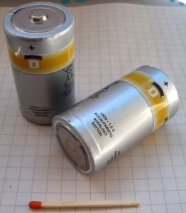
Figure 1: Picture of a Standard D-Cell (Wikipedia).
I am looking at supporting an Uninterruptible Power Source (UPS) that uses twelve D-size alkaline batteries for its energy source. Telecom service providers like D-size alkaline batteries because their subscribers can purchase them at many local grocery stores. They contain no harmful material and can be tossed in the trash. Service providers currently use a Sealed Lead-Acid (SLA) batteries. SLA batteries are not as widely available and and they contain lead, which must be recycled. However, SLA batteries are convenient because you only need one battery and it is fairly compact.
I thought it would be useful to show you the kind of mathematics that goes into evaluating a battery for use in a UPS application. This is my first application for a D-size batteries. My only contact with them goes back to the late 80s when my children had a CD player that used six D-size batteries. I just remember the batteries as being really big.
Background
Size of a D-Battery

Figure 2: Mechanical Drawing of a D-Size Battery.
Figure 2 shows a dimensioned drawing for a D-size battery. D-size batteries are the largest of the cylindrical batteries that are commonly available in grocery stores in the United States. In addition to being large in volume, they are also fairly heavy at 144 grams (5.1 ounces).
The primary reason that some service providers want to use D-size batteries is to ensure that their customers have easy access to replacement batteries. In the US, D-sized batteries are available at many stores (e.g. grocery, gas stations, department, hardware, automotive, etc). However, SLA batteries are not nearly as available − people usually buy them online or at some hardware stores. However, hardware stores are not nearly as common as grocery stores or gas stations.
Figure 3 shows how the D-size battery compares in size with other commonly seen battery sizes.

Figure 3: Comparison of Common Battery Sizes (Wikipedia).
The use of D-size batteries for backup power in Fiber-to-the-Home (FTTH) applications has been done before. Marconi used them for an early system. For reasons that I have never fully understood, that system was not commercially successful. However, those folks (like George BuAbbud) got a lot of things right in their design. It was a case of being a little too far ahead of where the market was.
Critical Battery Voltages
There are three battery voltage specifications that will be important for our discussion.
- Nominal Cell Voltage (VNom)
- This is the labeled battery voltage. For an alkaline battery, it is 1.5 V.
- Open Circuit Voltage (VOC)
- The open circuit voltage of a battery is the cell voltage of a fully charged battery with no load. For an alkaline battery, this voltage varies from 1.50 V to 1.65 V. The variation is caused by minor differences in concentrations of the materials used in the specific battery.
- Cutoff Voltage (VCO)
- The cutoff voltage is the cell voltage at which the battery is considered fully discharged.
For the discussion to follow, I will assume that VOC = VNom.
Energy Capacity
One of my tasks is to estimate the run-time of an Optical Network Terminal (ONT) when it is powered by twelve D-size batteries connected in series. The ONT is in backup mode and it will apply a constant load of 9 W to the battery string. My analysis will be based on Figure 4 from this battery specification.

Figure 4: Run-Time of a D-Size Battery As a Function of Load Current and Cut-Off Voltage.
Capacity Retention
Most of the work I do involve Telcordia specifications that mandate a backup time of 10 hours from a new battery and 8 hours from an aged battery. Thus, I plan on replacing the batteries when they have lost 20% of their capacity. The capacity loss from an alkaline battery is often stated to be 3 %/year (Figure 4 - Source).

Figure 5: Alkaline Capacity Degradation with Time.
Analysis
Battery Capacity as a Function of Cut-Off Voltage
Approach
My analysis will be very similar to that performed in this blog post on laser slope efficiency. I am most interested in determining the run time of this twelve-battery pack as a function of the cut-off voltage. The cut-off voltage is important to me because my power supply can only run down to ~10 V, which means my cut-off voltage will be  .
.
My analysis approach is simple.
- Digitize the curves in Figure 4 using Dagra.
- Create a two-dimensional interpolation of the digitized data from Figure 4 using Mathcad.
- Create a graph of run-time versus cut-off voltage.
Digitized Version of Figure 4
Figure 6 shows my digitization process.

Figure 6: Digitized Version of Figure 4.
Figure 7 shows how my digitized data looks when plotted in the format of Figure 4. They look identical.

Figure 7: Plot of My Digitized Data.
Generate 2-Dimensional Interpolation
Figure 8 shows the Mathcad program that I used to perform the 2-dimensional interpolation.
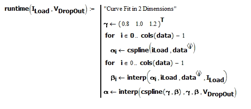
Figure 8: 2-Dimensional Interpolation.
Plot of Run-Time Versus Cut-Off Voltage
Figure 9 shows my graph of run-time versus cut-off voltage. My chart of battery performance assumes a constant load current. Because the battery voltage is always reducing and my ONT's power supply draws a constant power level (i.e. switched mode power converter), the current into my ONT is always varying. I will approximate this current with an average value.

Figure 9: Run-Time Versus Cut-Off Voltage.
This chart shows that I will have no problem meeting my 10 hour run-time requirement with a cut-off voltage set at 0.833 V per battery. I can even raise my power supply's cut-off voltage a bit if that will reduce my product cost.
Replacement Time
The replacement time is determined by the 3 % loss of capacity per year. Since I must replace the battery when the loss is 20 %, this means that I will get 6.66 years of service from this battery string before I must replace it. I typically expect to replace batteries every five years. So the D-size alkaline batteries have plenty of retained capacity.
Conclusion
The D-size alkaline battery can be an effective backup energy source for an ONT. My analysis here was strictly technical, but ultimately it will be economics that determines whether the market moves this way. I still have this analysis to perform.


 , which I illustrate in Figure 5(B).
 .
.