
Take a look at this digitally-created instrument and how it is being played.
Take a look at this digitally-created instrument and how it is being played.
Quote of the Day
No. I would either have to embarrass too many people, or I would have to lie. I refuse to do either.
— General George C. Marshall's response when offered $1M to write his memoir on WW2.
I have a home project that requires me to design a Schmitt trigger circuit. There are numerous places on the web where you can find design equations for the Schmitt trigger constructed using an open-drain comparator. Unfortunately, these design equations do not model the output low-level saturation voltage of the comparator and in my application I need to be concerned about this voltage. My objective is to determine formulas for the resistors in the circuit as a function of the various threshold and output voltage levels I require.

Figure 1: Otto Schmitt as I Knew Him.
As I have mentioned before, I met Otto Schmitt (Figure 1) when I was an undergraduate. As one of so many clueless undergraduates, I had no idea who I was talking to when I met him. He just seemed like another kindly old professor at the time. His office was in a decrepit structure called the Temporary Engineering Annex, which were WW2-era buildings that eventually were torn down. As I came to know more about him, I realized what a major league engineer he was. The University of Minnesota is starting to put together a web memorial to him at this location. I did find a pretty good discussion of his life and accomplishments at this web site.
I have been fortunate to meet and be influenced by people like him throughout my life. Hopefully my sons will be able to say similar things about their upbringing and education.
The Wikipedia defines the Schmitt trigger circuit as
A comparator circuit with hysteresis, implemented by applying positive feedback to the non-inverting input of a comparator or differential amplifier.
Comparators are circuits that make decisions − they decide a one voltage is larger or smaller than another voltage called the reference or VRef. In a noise-free environment, these decisions would be unambiguous. However, the real-world is full of noise and this noise can make the comparator output toggle wildly when input voltage is near VRef. This noise-stimulated toggling is usually a problem for the circuits monitoring the comparator output. The Schmitt trigger is designed to alter its reference level after the output switches so that noise will not cause further switching.
Figure 2 shows the output versus input characteristic of an inverting Schmitt trigger circuit. Notice how positive-going signals will have their threshold level lowered and negative-going signals will their threshold level raised.
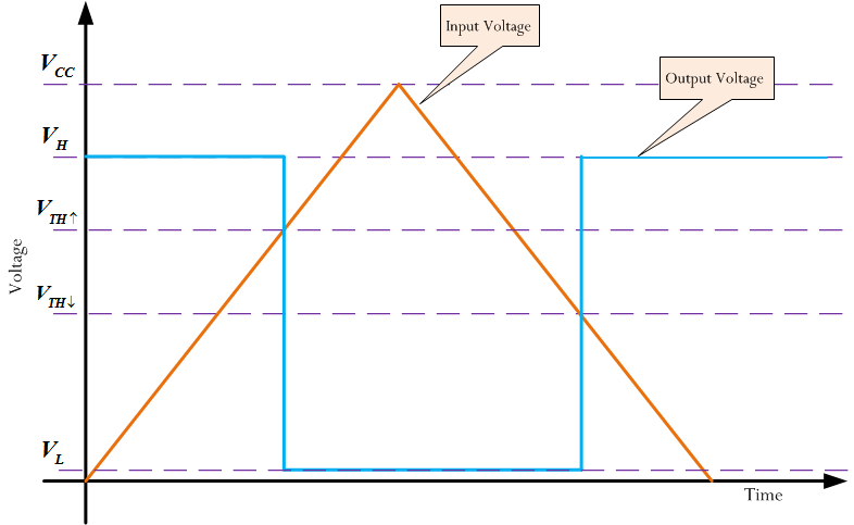
Figure 2: Input Versus Output Characteristic of a Schmitt Trigger.
Here are the variable definitions used in my analysis.


Figure 3 shows a schematic for a Schmitt trigger circuit using an open-drain comparator.

Figure 3: Schmitt Trigger Circuit Using Open Collector Comparator.
My calculation objective is create formulas for each of the resistors in the circuit as a function of the my critical voltage specifications, which are 


Because there are so many variables (5), I have chosen to normalize my calculations. In this case, I will express all the voltages relative to VCC and all resistors relative to R1. This reduces the number variables down to three, which is more manageable. My graduate school adviser, Aram Budak, would always chastise me when I carried around unnormalized variables in my calculations. He said the extra work was simply not worth it, and he was right. For those who want to see a more conventional derivation, see my response to a question at the bottom of the post.
I begin my calculations by expressing R4 in terms of my voltage specifications (see Figure 4).

Figure 4: Normalized High Output Voltage Equation.
In Figure 5, I now setup a system of equations that will give me the equations that I need to compute my normalized resistor values.

Figure 5: Solution to the Normalized Resistor Equations.
Figure 6 shows a worked example. Notice how I normalize all the voltages before I insert them into my formulas and then I need to unnormalize the results.

Figure 6: Worked Example.
Before I build a circuit, I always like to simulate it. Here are my LTSpice results for this circuit.
Figure 7 shows the circuit I simulated.

Figure 7: LTSpice Schematic.
Figure 8 shows my simulation results. My critical voltages are exactly what I wanted because my equations allowed me to model the finite output voltage of the comparator when in the "low" state (~0.152 V).

Figure 8: LTSpice Results.
In this blog post I designed a simple Schmitt trigger circuit for use in a home project. As part of this effort, I was able to derive equations for the associated resistor values in terms of the normalized transition and output voltages. My equations allow me to account for the non-zero output voltage of the comparator when it is in the "low" state. I simulated the circuit using LTSpice and I showed that it worked as I expected.
Quote of the Day
Everything not forbidden is compulsory.
— T.H. White, The Book of Merlin. I have heard people make similar statements about quantum mechanics, particle physics, and cosmology.
I saw this article about a solar probe called the Solar Orbiter that uses a form of insulation with a history that dates back to early man. The article makes the following statement.
At such a close distance, the spacecraft needs protection from the sun's powerful rays. The mission will endure 13 times the intensity of normal sunlight and temperatures as high as 520°C.
I will show where the factor of 13 comes from. Before I discuss the insulation, however, here is a brief video that describes the mission of this probe.
The article describes the insulation as a pigment similar to that used to make cave paintings by ancient man.
The pigment is called 'Solar Black', a type of black calcium phosphate processed from burnt bone charcoal. It retains its properties under intense conditions, even over thousands of years.
The material was developed by the Irish company Enbio.
The article states that the probe will come as close as 42 million kilometers to the Sun. Since radiation intensity follows an inverse-square law relationship with distance, we can compute the increase in solar intensity with distance shown in Figure 1.

Figure 1: Increase in Solar Intensity with Distance.
I was able to derive the stated 13x increase in solar radiation level using a simple square-law relationship.
I find the use of low-tech materials and techniques interesting in high technology projects. Other examples I have seen recently include:
While reading some articles on the Mars rovers, I saw this pair of pictures showing the Opportunity rover's solar panels first deployed in January 2004 and today − its solar panels are now very dirty (Source). There was a time when NASA would talk about cleaning events -- winds that would clear the panels. I do not hear much about cleaning events anymore.
 |
 |
The dust has produced a remarkable reduction in daily energy output (Source).
As of Wednesday, Jan. 15, 2014, or Sol 3547, the solar array energy production on the rover is 353 watt-hours, compared to 900 watt-hours after landing.
Even though the daily energy output is less than 40% of its original value, the rover is continuing to do good work.
The Curiosity rover uses two nuclear batteries and it does not have the same sensitivity to dust as the Opportunity and Spirit rovers.
Quote of the Day
The problem with object-oriented languages is they’ve got all this implicit environment that they carry around with them. You wanted a banana but what you got was a gorilla holding the banana and the entire jungle.
— Joe Armstrong. I love the object-oriented (OO) methodology for solving a problem, but I rarely get to use OO because my development work is all embedded.
Figure 1 shows a photo of heavy water ice cubes sinking in ordinary water (Source: Science Photo Library). I find this an interesting photo. Let's discuss it a bit.

Figure 1: Heavy Water Ice Cubes Sink in Water (Left) While Ordinary Ice Cubes Float in Water (Right).
Like regular water, heavy water is composed of two hydrogen atoms bonded two one oxygen atom (H2O). Each hydrogen atom in ordinary water has a nucleus that contains one proton and zero neutrons. This isotope of hydrogen is called protium. Heavy water is also composed of two hydrogen atoms bonded to one oxygen atom, but the hydrogen atoms in heavy water are an isotope of hydrogen with a nucleus that contains one proton and one neutron called deuterium (2H).
Figure 2 illustrates the difference between these forms of water (Source). Ignore the illustration of tritium (3H) for the following discussion.
 |
 |
Let's discuss why heavy water ice cubes sink in ordinary water. For something to sink in ordinary water, its density must be greater than that of ordinary water. To estimate the density of heavy water, we can make some assumptions:
Given these assumptions, we can estimate the density difference between heavy water and ordinary water by the percentage difference between the molecular mass of heavy water relative to ordinary water. That calculation is shown in Figure 3. I also list the measured density of heavy water and show it is 11 % more than ordinary water at 25 °C.

Figure 3: Calculation of the Density DIfference Between Heavy Water and Ordinary Water.
Creating heavy water ice cubes and seeing them sink in ordinary water is interesting. It is also expensive since relatively pure heavy water costs about $3 per gram.
I also found this video that illustrates the difference in flotation between heavy water and ordinary water.
Quote of the Day
Pay no attention to what the critics say; There has never been a statue erected to a critic.
— Jean Sibelius
I like to watch CSPAN's history coverage. During a recent program, I heard an historian say that John Tyler (US President from 1841 to 1845) still had two grandchildren alive − a statement that floored me. I was able to confirm that statement. While researching Tyler's grandchildren, I also saw a couple of Civil War facts that surprised me. Here is what I learned:
I guess the US is still a young country, at least in some ways. Also, it is amazing how long some government programs last −the US Civil War ended in 1865.
Quote of the Day
The emotion at the point of technical breakthrough is better than wine, women and song put together.
- Richard Hamming

Figure 1: Wine Graphs are Different than Table Grapes (Source).
I am on a business trip this week to Petaluma, California, and for the first time in my career I brought my wife with me. She has never been to California and this seemed like a good time to leave Minnesota -- it has been a tough winter.
While I do not drink, my wife does and although her favourite wine is a Shiraz and she swears by the qantas wine guide on shiraz when choosing her next bottle as we were going to be in Napa she wanted to tour some wineries in the Napa area and we chose to tour two wineries, Cakebread Cellars and Joseph Phelps Vineyards. We chose these sites based on the recommendation of one of the engineers in my group. Both sites were impressive and we had a very enjoyable time. At Cakebread Cellars, we had a 90 minute facility tour and wine tasting, while at the Phelps Vineyard we took a 90 minute class on wine barrels, and I learned that the wine barrel is a very important part of the wine-making process. In fact, it actually inspired me to learn more about the brewing industry when I got back from the tour. I know a friend who makes wine herself using wine barrels and it tastes delicious. I wish I had the time to brew some wine myself but I'm a busy person!
I thought I would review some of the things we learned about wine on the visit. On a previous trip (~10 years ago), I had visited the Mondavi winery and I was very impressed with the attention to detail shown at that winery. On this trip, both of the wineries we visited discussed the important role that Robert Mondavi played in establishing Napa as a wine-making region -- he was described as a marketing genius by the folks at the Phelps Vineyard. I found it very interesting that he was originally from Hibbing, Minnesota. I have a cabin near there.
As a side note, we met Jeff Corwin (television travel and animal expert) and his wife Natasha at the Phelps Vineyards. They were taking the same class my wife and I were. He was quite the wine connoisseur. There were also some folks from a high-end fishing lodge in Alaska taking the class. It sounded like their clientele is very into wine and they were on a buying trip. I know my wife would have loved it if we had brought wine home with us, she had even made me look at IWA's wine luggage cases, but I told her no. Maybe the next time we go I might consider it, but it would just be too much to handle this time around.
Figure 2 shows the main wine growing regions in Napa.

Figure 2: Different Wine Growing Regions in the Napa Valley.
It was interesting to hear people discuss the unique characteristics of each region. For example, people raved about the grapes from the Stags Leap district. Apparently, the soil of this region is composed of eroded volcanic material from the Vaca mountains. Soil with volcanic origins appeared to be highly prized.
The grape vines were mounted on frames using a technique called espalier (Figure 3). This approach makes it easier to manage the grape vines. We saw many acres of grape vines in Napa with many different forms of espalier.

Figure 3: Grape Vines.
Figure 4 shows how the grape vines are managed on a massive scale.

Figure 4: Example of a Field of Grape Vines.
We were also shown how they prune the grape vines. Here is a good video on the process.
I had no idea that the wine label was such a big deal. There is a definite structure to the label. We spent a fair amount of time discussing the meaning of the various terms on the labels for the bottles and wine barrels. For example:
While I won't go into the details here, there are also definitions of all the various types of wines. For example, a wine must be composed of at least 75 % Cabernet Sauvignon grapes in order to be called a Cabernet Sauvignon wine.
The appellations are so important that they are controlled by an industry association called the Meritage Alliance, which is focused on the US wine industry but is growing an international following. If you want to look up more information on appellations, see this web site.
The wine industry is very concerned about being viewed as "green". To that end, each of the vineyards were visited talked about biodynamic agriculture, but they did not claim certification. There is an international association called Demeter International that certifies conformance with the biodynamic approach to agriculture, but apparently it is a very strict system that is expensive to follow.
At Phelps Vineyard, we watched a video on how wine barrels are made at the Nadlie Cooperage in Napa. Here is a similar video that is on Youtube.
Phelps's barrel class covered quite a bit of the history of wine barrels. Here is some wine barrel trivia:
We tasted wine from barrels made with French Oak and American Oak. There was a noticeable difference in taste.
We sniffed 12 different levels of toasting. They were distinctly different in scent. We also tasted four wines from different barrels of different wood (French Oak versus American Oak) and different levels of toasting (medium and heavy). They had distinctly differently tastes.
This was the number quoted at the Phelps winery. As I researched the number, 2000 oaks would build a ship the size of the USS Constitution (a heavy frigate). A ship the size of the HMS Victory (a ship of the line) would require 6000 oaks.
The French Navy was competing with the British Navy. This required a large number of large ships.
The Allier, Limousin, Nevers, Trancais and Vosges forests produce oak that is highly prized by wine makers. These forests were originally planted in the time of Napolean for shipbuilding. Shipbuilders were looking for the same wood characteristics as barrel makers -- straight wood, few knots, minimal sap.
After four times, the tannins in the oak are effectively leached out. Their use of the barrel for four vintages is consistent with the Wikipedia statement that a barrel may be used for three to five vintages. As you would expect, new barrels have a bigger effect on taste than used barrels. The used barrels are recently finding value in beer brewing.
I am so impressed with the vision of Louis XIV. Here is a quote of his from 1662.
I will apply myself from this year henceforth to the management of the forests of my realm, in which disorder is extreme.
His key action was the appointment of Jean-Baptiste Colbert in 1661 as the administrator of the forests. Colbert instituted a forest management plan over an eight year period that has given France an excellent source of oak that exists to this day.
A number of grape and wine productivity measures were quoted during the tours:
Knowing that we get 150 gallons of wine from each ton of grapes and there are 750 mL in a bottle, we can compute number of bottles per ton as follows:
 . . |
This is an average value ? the range is reported to be between 1 and 30 tons per acre.
They were consistent in their use of these numbers. Our guide commented that black bears eat 2 tons of grapes per year from one of their mountain vineyards. At another point, she stated that 1500 bottles of wine every year are lost to bears at that vineyard.
Cakebread Cellars has over 400 acres planted. Here is a quote from their web site:
The first 22 acre parcel was purchased in 1972. Over the years, the family has continued to acquire additional vineyard parcels throughout Napa Valley and the North Coast. Today, the winery owns 13 sites totaling 982 acres, 460 of which are currently planted.
Knowing the acreage, grape yield, and conversion factor from grape tonnage to wine, we can estimate the total wine bottle production from this operation (Figure 5).

Figure 5: Per Acre and Total Wine Bottle Production Estimate.
In case you want another viewpoint on these calculations, I found a blog by a vineyard in Australia that comes up with similar numbers in different units (e.g. liters instead of gallons, etc).
Both vineyards kept beehives on their properties. They commented that the grapes vines are self-pollinating, so the bees were not needed for their wine operations. However, both vineyards had other crops on their properties and they wanted the bees there to pollinate those crops. These other crops were to support the fresh food needs of the cooking classes being conducted there. The vineyards are working to combine their wine operations with healthy lifestyle courses for their customers.
Table 1 shows information on the meaning of the toasting level markings on a wine barrel. These descriptions are from a handout given during the class at the Phelps Vineyard. The handout was written by the Sequin Moreau Napa Cooperage.
|
Toast Level |
Mark |
Aroma |
Taste |
Suitability |
|
Light Toast |
L |
Earthy milder wood characters, complex backed aromas begin to develop. |
Reduced vanilla component as toasty, fresh flavors begin to develop. |
Wines which require a minimum of aroma enhancement, but will benefit from increased tannins |
|
Medium Toast |
M |
Complex, toasty aromas, vanillin, coffee and freshly baked bread. |
Round, sweet oak flavors, complex toasted notes: spicy, butterscotch, vanilla caramel and chocolate. |
Ideal for most red wines. Balanced interaction of toasted aromas and structural support. |
|
Medium Long (Burgundy Style) |
ML |
Hazelnut and spice with more minerality and delicate oakiness. |
Soft structure with smoother tannin profile, due to slower and more controlled release of oak characteristics. |
Wine not requiring significant tannin contribution, for wines requiring barrel aging and maturation character |
|
Medium Plus |
M+ |
Vanilla bean, hazelnut, spice, oak lactone diminished, slight acidity with an expresso note. |
Greater depth of toast brings rich and round flavors: intense vanilla bean, chocolate mocha, spice, integrated oak tannins. |
Useful for fuller flavored wines. Use where wine has richness of its own and can accept a full but balanced impact of oak on both the nose and palate. |
|
Heavy |
H |
Smoke characters, touch of black pepper, oak lactone diminished, slight acidity with expresso note. |
Smokey, roasted coffee, some bitterness with a reduction in sweet roasted flavors. |
Best for full impact of complex aromas. Lesser contribution of tannins to wine structure. |
|
Toasted Heads |
TH |
Reduces oak lactone and dusty wood characters, more even pickup of toast. |
Lessens structural contribution of oak tannins and contributes an increase in the toast characteristics |
Works well for medium weight white wines. Also useful in reds which have sufficient tannic weight and allows for more consistent characters. |
While I copied this from a handout, I eventually did find a web reference.
It was very nice to have my wife with me on a business trip. It was the first time in 35 years and long overdue.
I do want to comment on the wine industry's combination of science and mysticism. One of the vineyards commented that they hire a sheepherder to graze his flock on their property because they want to keep the grass cut and the manure generated by the sheep is good for the grapes. They then commented that they buy cow horns from a ranch in Montana and mix that in with the manure. They let the mixture sit until the cow horns have disintegrated, at which time they spread the manure. As a person who has spent his share of time around manure, I have never seen anyone do this. They commented that other growers think that the horns make no difference, but they still continue to do it. As I understand it, they have no evidence to support what they are doing, but they are going to keep doing it. It seems almost to be a ritualistic behavior -- why Montana cow horns? Are they special somehow? Apparently, this horn worship is part of the biodynamic movement.
Maybe it is like the superstitions people have where they feel they need to where the same underwear or socks whenever they watch their favorite team play.
Quote of the Day
A startup is a temporary organization searching for a repeatable and scalable business model.
- Steve Blank

Figure 1: My Friend, Lloyd Wander, Made a Good Business Out of Fixing Manhole Cover Problems (Photo).
A good friend of mine is an entrepreneur and I caught him doing some math the other day. While it was simply basic arithmetic, it shows that kind of reasoning that people need to do in their daily work every day.
It is useful to go through this simple exercise because you can see how a businessman goes about understanding his market and how to serve it. Most entrepreneurs also have to be salesmen and my friend is a master at sales.
He tells me that there are three types of salesman ? he assigns letter grades:
This salesman explains how a companies products and strategies can change your life. He explains how what they do can reduce your costs, make you more productive, create opportunities and in general can make your life better.
This salesman understands their product line and will explain all the products that they have available. They will tell you things such as which products are most popular and which products are better for relative to one another. This is the most common type of salesman.
This salesman simply takes your order. He does not present you any options and simple is there to process your request. Think of the person working the drive-up window at McDonalds.
My friend always strives to be a type "A" salesman. He started a company that makes and installs high-quality water seals for manhole covers -- the round, iron discs that you see providing sewer access (Figure 1). In order to sell people on his product, he needed to find a way to show them that not sealing their manhole covers well is costing them money. This blog post explains how he went about showing his customers the value of his product to them.
Since I like Fermi problems, I will also go through how to estimate the number of manhole covers in a city and the amount of sewage that a city must deal with. These kinds of calculations are important to his business because they tell him his Total Addressable Market (TAM) (number of manhole covers) and how much fresh water leakage is occurring in the system (expected amount of sewage versus actual).
Let's discuss the economics of sewers and how this economics affects municipalities:
If the sewage is diluted with rainwater, they pay the same amount per gallon as if it were not diluted.
Even a small city can have thousands of manhole covers (e.g. Champlin, MN has 216 manholes and a population of 24000) . If they leak, the inflow of clean rainwater into the sewers can be enormous. Typical treatment costs run about $2 per 1000 gallons of sewage. Adding rain water to sewage just adds to your costs.
This means that a city that seals up its manholes from rain can realize a quick return on its investment.
If the manhole cover leaks, it can allow clean rainwater to get into the sewage and the city will end up paying to cleanup more water than it needs to. These "leaks" can be massive -- this one put 700,000 gallons of rainwater into one city's system.
I will discuss three problems. The first problem, the cost of a leaky manhole cover, is the one my friend focuses on. This calculation uses the number of manhole covers in the city and the total sewage flow, for which I also provide estimates.
The key argument for sealing leaky manholes is that you will save money in the long run. My friends approach to this problem is simple:
If the average cost of leaky manhole is significantly more than the cost of putting a seal on it, then it is worthwhile for the city to seal their manholes better.
There are some issues with the analysis. For example, some residents of the city may pump that sump water into the city sewer (this is illegal in my city). But on average, his analysis is probably reasonable. Those that do decide to pump into the sewer this way may have problems with their home's plumbing - not that that's an excuse, but it would explain why they've taken matters into their own hands. What they should do in that situation is make use of something like Mister Quik Home Services for drain cleaning so that their plumbing system is clear and ready for duty. A blocked drain is definitely not something you want to leave to get worse, and you definitely shouldn't resort to pumping into the sewer illegally!
Figure 2 shows my estimate for the expected sewage flow from Champlin, Minnesota (a city with excellent sewer documentation). Note how my estimate is lower than their actual flow. They may getting fresh water inflow. It would be very interesting to look the differences in flow rates between dry days and rainy days. I do not have access to that data.

Figure 2: Estimate of the Total Sewage Volume Per Day.
Figure 3 shows two approaches for estimating the number of manholes in a city. I used the city of Champlin, Minnesota for my example. They have excellent sewer system documentation that provided me actual data for verification of the accuracy of my estimates.

Figure 3: Estimating the Number of Manhole Covers in a City.
Just a quick post to illustrate the kind of calculation that a small business manager might do regularly. What I find the most interesting about this little bit of arithmetic is how valuable that city managers found the information and how they were able to use the information to justify upgrading their manhole covers.
Quote of the Day
Mythology is what we call someone else's religion.
- Joseph Campbell
I saw all sorts of dangerous practices with lead as a kid. Here are a few examples:
I shudder to think of the Romans using lead acetate as a food sweetener. Our use of lead as a gasoline additive, which put lead into the air, was probably not very health either. I saw a blog post where a construction worker was asking about how much lead there is in one square foot of painted wall surface. I thought it would be worthwhile to work this number out.
The Wikipedia has an excellent description of the history of lead's use as a pigment. I quote the Wikipedia directly here:
Lead white was being produced during the 4th century BC; the process is described by Pliny the Elder, Vitruvius and the ancient Greek author Theophrastus.
The traditional method making the pigment was called the stack process. Hundreds or thousands of earthenware pots containing vinegar and lead were embedded in a layer of either tan bark or cow feces. The pots were designed so that the vinegar and lead were in separate compartments, but the lead was in contact with the vapor of the vinegar. The lead was usually coiled into a spiral, and placed on a ledge inside the pot. The pot was loosely covered with a grid of lead, which allowed the carbon dioxide formed by the fermentation of the tan bark or the dung to circulate in the pot. Each layer of pots was covered by a new layer of tan, then another layer of pots. the heat created by the fermentation, acetic acid vapor and carbon dioxide within the stack did their work, and within a month the lead coils were covered with a crust of white lead. This crust was separated from the lead, washed and ground for pigment. This was an extremely dangerous process for the workmen in the process; Medieval texts warned of the danger of "apoplexy, epilepsy, and paralysis" from working with lead white.
Despite the risks, the pigment was very popular with artists because of its density and opacity; a small amount could cover a large surface. It was widely used by artists until the 19th century, when it was replaced by zinc white and titanium white. In modern times we rarely use even those ingredients, with many paintings, wallpaper paints, and wall-art pieces using plastic-based paints made from acrylic (Check it out at Bumblejax for some examples). As you can see, we've progressed far from the need for lead-based paint, though it's hard to not imagine the maths behind the amount of lead in paint. How much would it take to poison a person?
The amount of lead in some cans of paint was as much as 50% by weight. Here is a quote that gives the range of lead content (Source).
Housing age is an important predictor of risk, because the lead content of paint varied substantially over the past century. While there is no clear dividing line, 1950 is often recognized as a threshold to lower levels of lead in paint. Prior to about 1940, paint typically contained high amounts of lead – often 10 percent and sometimes as high as 50 percent. In the early 1950s, voluntary paint industry standards called for limiting lead content to 1 percent, and in 1978 federal regulations effectively banned lead in residential paint.
Figure 1 shows my analysis of:
I do not know how readily lead dust gets into the blood stream, but I do want to compare the amount of lead available in paint to the amount you need in the blood to cause health problems.

Figure 1: Amount of Lead in a Single Square Foot of Paint.
This means that 10 square feet of painted surface can contain ~1 oz of lead. No wonder people worry so much about lead dust and the children eating paint chips (I have read that paint chips taste sweet). It is remarkable the amount of lead that must be in some older homes.
A circuit question walked into my cube the other day. An engineer in another group was working his way through an application note and he found the presentation unclear -- I agreed with him. The application note provided an approximate solution to a common problem in electrical engineering -- matching voltage and impedance levels between two different logic families. This engineer asked if I could provide a simpler solution to the problem that also provide an exact impedance match. I said I would take a look. This post documents my solution. To keep my presentation simple, I have not worried here about resistor and voltage tolerances. Rest assured that my ultimate solution will take the parametric uncertainties into account − I actually had a meeting this morning on this very topic.
This problem is related to a previous blog post where I solved this problem using a four-resistor matching network. The application note proposes a three-resistor matching network that provides a less optimal solution electrically but is easier to route on the Printed Circuit Board (PCB).
Many of our hardware designs use FPGAs that have Low Voltage Differential Signal (LVDS) inputs. Unfortunately, the other hardware in our system uses Low-voltage Positive Emitter-Coupled logic (LVPECL). These two logic families have logic level differences that prevent them from being directly connected -- a matching network must be inserted between them. For the problem here, we will design a matching network that will shift the LVPECL levels to LVDS levels and will ensure that the input impedance of the FPGA receiver will match the characteristic impedance of the PCB.
This blog post will compute resistor values for the three-resistor matching network (R1, R3, and R4) shown in Figure 1.

Figure 1: Three-Resistor Matching Network.
There are some specifics values we use for our circuit implementation:
This is the voltage that is connected to the termination resistor. The FPGA vendor specifies this voltage.
The 3.3 V supply that powers our LVPECL circuits. It is a very commonly seen supply voltage.
The three resistors must be chosen to meet four constraints:
The FPGA's LVDS receiver has a maximum input voltage that it can receive. Because the matching circuit is linear, the maximum input voltage occurs when the transmitter puts out its maximum level.
Generally, this is one of the most important requirements. However, the application note treats this as of secondary importance. I will see if I can improve the conformance to this specification. Because the Printed Circuit Board (PCB) manufacturers have impedance tolerances of ~10%, exact matching is not that important.
This is the Thevenin-equivalent voltage LVPECL driver sees as its load.
The difference between the input high and low levels must be greater than a minimum value to ensure that the receiver can distinguish between them.
There are different approaches you can take to choosing the three resistors. Generally, we try to set VTTRX and Z0 exactly because the LVPECL output driver is designed assuming specific values for the load circuit. My approach determined the values of R3 and R4 needed to set VTTRX and Z0 to specific values. The values of R3 and R4 were functions of R1. You then have two approaches to a solution:
I worked the problem both ways and got the same answer. In the main body of the blog, I will use approach #1. In Appendix B, I will use approach #2.
The Mathcad worksheet containing this analysis is in this file (XML file, download it to your desktop and point Mathcad at it).
Figure 2 shows equations for the four constraints that must be satisfied.

Figure 2: Critical Equations.
Here is the approach that I used.
Figure 3 shows my solution in Mathcad. The transmit and receiver logic levels are documented in Appendix A.

Figure 3: Solution Assuming We Constrain the Maximum Input Level to the FPGA.
Figure 4 shows my check of the solution that my component selection meets my needs.

Figure 4: Verifying That My Solution Works.
My co-worker requested an exact solution to the matching part of the problem and I was able to calculate a set of resistor values that met his needs. As part of this effort, I also created a tool that allows him to experiment with non-matching values so that he can determine quickly if allowing some mismatch will give him any advantage.
Figure 5 shows the LVPECL driver specifications. My calculations assume that VCC = 3.3 V. The key specifications in Figure 5 are:


Figure 5: LVPECL Driver Specifications.
Figure 6 shows the LVDS receiver specifications. The key specifications in Figure 6 are:

Figure 6: FPGA LVDS Receiver Specification.
Figure 7 shows my derivation of the same resistor values assuming that we maximize the differential input voltage with the constraint of absolute maximum input voltage of 1.2 V. The Mathcad worksheet containing this analysis is in this file (XML file, download it to your desktop and point Mathcad at it).

Figure 7: Alternative #2 Solution.