The problem with object-oriented languages is they’ve got all this implicit environment that they carry around with them. You wanted a banana but what you got was a gorilla holding the banana and the entire jungle.
— Joe Armstrong. I love the object-oriented (OO) methodology for solving a problem, but I rarely get to use OO because my development work is all embedded.
Introduction
Figure 1 shows a photo of heavy water ice cubes sinking in ordinary water (Source: Science Photo Library). I find this an interesting photo. Let's discuss it a bit.
Figure 1: Heavy Water Ice Cubes Sink in Water (Left) While Ordinary Ice Cubes Float in Water (Right).
Background
Like regular water, heavy water is composed of two hydrogen atoms bonded two one oxygen atom (H2O). Each hydrogen atom in ordinary water has a nucleus that contains one proton and zero neutrons. This isotope of hydrogen is called protium. Heavy water is also composed of two hydrogen atoms bonded to one oxygen atom, but the hydrogen atoms in heavy water are an isotope of hydrogen with a nucleus that contains one proton and one neutron called deuterium (2H).
Figure 2 illustrates the difference between these forms of water (Source). Ignore the illustration of tritium (3H) for the following discussion.
Figure 2: Forms of Hydrogen and Their Formation into Heavy Water and Ordinary Water.
Analysis
Let's discuss why heavy water ice cubes sink in ordinary water. For something to sink in ordinary water, its density must be greater than that of ordinary water. To estimate the density of heavy water, we can make some assumptions:
Atoms of heavy water and ordinary water are the same size
Heavy water ice and ordinary ice form exactly the same crystal structure.
Given these assumptions, we can estimate the density difference between heavy water and ordinary water by the percentage difference between the molecular mass of heavy water relative to ordinary water. That calculation is shown in Figure 3. I also list the measured density of heavy water and show it is 11 % more than ordinary water at 25 °C.
Figure 3: Calculation of the Density DIfference Between Heavy Water and Ordinary Water.
Pay no attention to what the critics say; There has never been a statue erected to a critic.
— Jean Sibelius
I like to watch CSPAN's history coverage. During a recent program, I heard an historian say that John Tyler (US President from 1841 to 1845) still had two grandchildren alive − a statement that floored me. I was able to confirm that statement. While researching Tyler's grandchildren, I also saw a couple of Civil War facts that surprised me. Here is what I learned:
I guess the US is still a young country, at least in some ways. Also, it is amazing how long some government programs last −the US Civil War ended in 1865.
Posted inMilitary History|Comments Off on Presidential and Civil War Trivia
The emotion at the point of technical breakthrough is better than wine, women and song put together.
- Richard Hamming
Introduction
Figure 1: Wine Graphs are Different than Table Grapes (Source).
I am on a business trip this week to Petaluma, California, and for the first time in my career I brought my wife with me. She has never been to California and this seemed like a good time to leave Minnesota -- it has been a tough winter.
While I do not drink, my wife does and although her favourite wine is a Shiraz and she swears by the qantas wine guide on shiraz when choosing her next bottle as we were going to be in Napa she wanted to tour some wineries in the Napa area and we chose to tour two wineries, Cakebread Cellars and Joseph Phelps Vineyards. We chose these sites based on the recommendation of one of the engineers in my group. Both sites were impressive and we had a very enjoyable time. At Cakebread Cellars, we had a 90 minute facility tour and wine tasting, while at the Phelps Vineyard we took a 90 minute class on wine barrels, and I learned that the wine barrel is a very important part of the wine-making process. In fact, it actually inspired me to learn more about the brewing industry when I got back from the tour. I know a friend who makes wine herself using wine barrels and it tastes delicious. I wish I had the time to brew some wine myself but I'm a busy person!
I thought I would review some of the things we learned about wine on the visit. On a previous trip (~10 years ago), I had visited the Mondavi winery and I was very impressed with the attention to detail shown at that winery. On this trip, both of the wineries we visited discussed the important role that Robert Mondavi played in establishing Napa as a wine-making region -- he was described as a marketing genius by the folks at the Phelps Vineyard. I found it very interesting that he was originally from Hibbing, Minnesota. I have a cabin near there.
As a side note, we met Jeff Corwin (television travel and animal expert) and his wife Natasha at the Phelps Vineyards. They were taking the same class my wife and I were. He was quite the wine connoisseur. There were also some folks from a high-end fishing lodge in Alaska taking the class. It sounded like their clientele is very into wine and they were on a buying trip. I know my wife would have loved it if we had brought wine home with us, she had even made me look at IWA's wine luggage cases, but I told her no. Maybe the next time we go I might consider it, but it would just be too much to handle this time around.
Wine Basics
Wine Growing Regions in the Napa Valley
Figure 2 shows the main wine growing regions in Napa.
Figure 2: Different Wine Growing Regions in the Napa Valley.
It was interesting to hear people discuss the unique characteristics of each region. For example, people raved about the grapes from the Stags Leap district. Apparently, the soil of this region is composed of eroded volcanic material from the Vaca mountains. Soil with volcanic origins appeared to be highly prized.
The Grapes
The grape vines were mounted on frames using a technique called espalier (Figure 3). This approach makes it easier to manage the grape vines. We saw many acres of grape vines in Napa with many different forms of espalier.
Figure 3: Grape Vines.
Figure 4 shows how the grape vines are managed on a massive scale.
Figure 4: Example of a Field of Grape Vines.
We were also shown how they prune the grape vines. Here is a good video on the process.
The Wine Label and Appellations
I had no idea that the wine label was such a big deal. There is a definite structure to the label. We spent a fair amount of time discussing the meaning of the various terms on the labels for the bottles and wine barrels. For example:
To put the name "Napa" on the label (called an "appelation"), the 85 % of the grapes used to make the wine must come from the Napa region.
For a California appellation, 100 % of the grapes must come from California.
For a county appellation, 75 % of the grapes used must be from that county.
The appellations are so important that they are controlled by an industry association called the Meritage Alliance, which is focused on the US wine industry but is growing an international following. If you want to look up more information on appellations, see this web site.
Eco-Friendly
The wine industry is very concerned about being viewed as "green". To that end, each of the vineyards were visited talked about biodynamic agriculture, but they did not claim certification. There is an international association called Demeter International that certifies conformance with the biodynamic approach to agriculture, but apparently it is a very strict system that is expensive to follow.
Making Wine Barrels
At Phelps Vineyard, we watched a video on how wine barrels are made at the Nadlie Cooperage in Napa. Here is a similar video that is on Youtube.
Phelps's barrel class covered quite a bit of the history of wine barrels. Here is some wine barrel trivia:
The wine barrel has a noticeable effect on the taste of the wine
We tasted wine from barrels made with French Oak and American Oak. There was a noticeable difference in taste.
The toasting of the wine barrel made a big difference in taste
We sniffed 12 different levels of toasting. They were distinctly different in scent. We also tasted four wines from different barrels of different wood (French Oak versus American Oak) and different levels of toasting (medium and heavy). They had distinctly differently tastes.
The Allier, Limousin, Nevers, Trancais and Vosges forests produce oak that is highly prized by wine makers. These forests were originally planted in the time of Napolean for shipbuilding. Shipbuilders were looking for the same wood characteristics as barrel makers -- straight wood, few knots, minimal sap.
Barrels can be used up to 4 times for making wine.
After four times, the tannins in the oak are effectively leached out. Their use of the barrel for four vintages is consistent with the Wikipedia statement that a barrel may be used for three to five vintages. As you would expect, new barrels have a bigger effect on taste than used barrels. The used barrels are recently finding value in beer brewing.
I am so impressed with the vision of Louis XIV. Here is a quote of his from 1662.
I will apply myself from this year henceforth to the management of the forests of my realm, in which disorder is extreme.
His key action was the appointment of Jean-Baptiste Colbert in 1661 as the administrator of the forests. Colbert instituted a forest management plan over an eight year period that has given France an excellent source of oak that exists to this day.
about 750 bottles of wine for every ton of grapes (assumes 750 mL bottles)
Knowing that we get 150 gallons of wine from each ton of grapes and there are 750 mL in a bottle, we can compute number of bottles per ton as follows:
.
An average of 4 tons of grapes per acre.
This is an average value ? the range is reported to be between 1 and 30 tons per acre.
They were consistent in their use of these numbers. Our guide commented that black bears eat 2 tons of grapes per year from one of their mountain vineyards. At another point, she stated that 1500 bottles of wine every year are lost to bears at that vineyard.
Cakebread Cellars has over 400 acres planted. Here is a quote from their web site:
The first 22 acre parcel was purchased in 1972. Over the years, the family has continued to acquire additional vineyard parcels throughout Napa Valley and the North Coast. Today, the winery owns 13 sites totaling 982 acres, 460 of which are currently planted.
Knowing the acreage, grape yield, and conversion factor from grape tonnage to wine, we can estimate the total wine bottle production from this operation (Figure 5).
Figure 5: Per Acre and Total Wine Bottle Production Estimate.
In case you want another viewpoint on these calculations, I found a blog by a vineyard in Australia that comes up with similar numbers in different units (e.g. liters instead of gallons, etc).
Bees
Both vineyards kept beehives on their properties. They commented that the grapes vines are self-pollinating, so the bees were not needed for their wine operations. However, both vineyards had other crops on their properties and they wanted the bees there to pollinate those crops. These other crops were to support the fresh food needs of the cooking classes being conducted there. The vineyards are working to combine their wine operations with healthy lifestyle courses for their customers.
Label Descriptions of Toasting
Table 1 shows information on the meaning of the toasting level markings on a wine barrel. These descriptions are from a handout given during the class at the Phelps Vineyard. The handout was written by the Sequin Moreau Napa Cooperage.
Table 1: Toasting Level Information.
Toast Level
Mark
Aroma
Taste
Suitability
Light Toast
L
Earthy milder wood characters, complex backed aromas begin to develop.
Reduced vanilla component as toasty, fresh flavors begin to develop.
Wines which require a minimum of aroma enhancement, but will benefit from increased tannins
Medium Toast
M
Complex, toasty aromas, vanillin, coffee and freshly baked bread.
Round, sweet oak flavors, complex toasted notes: spicy, butterscotch, vanilla caramel and chocolate.
Ideal for most red wines. Balanced interaction of toasted aromas and structural support.
Medium Long
(Burgundy Style)
ML
Hazelnut and spice with more minerality and delicate oakiness.
Soft structure with smoother tannin profile, due to slower and more controlled release of oak characteristics.
Wine not requiring significant tannin contribution, for wines requiring barrel aging and maturation character
Medium Plus
M+
Vanilla bean, hazelnut, spice, oak lactone diminished, slight acidity with an expresso note.
Greater depth of toast brings rich and round flavors: intense vanilla bean, chocolate mocha, spice, integrated oak tannins.
Useful for fuller flavored wines. Use where wine has richness of its own and can accept a full but balanced impact of oak on both the nose and palate.
Heavy
H
Smoke characters, touch of black pepper, oak lactone diminished, slight acidity with expresso note.
Smokey, roasted coffee, some bitterness with a reduction in sweet roasted flavors.
Best for full impact of complex aromas. Lesser contribution of tannins to wine structure.
Toasted Heads
TH
Reduces oak lactone and dusty wood characters, more even pickup of toast.
Lessens structural contribution of oak tannins and contributes an increase in the toast characteristics
Works well for medium weight white wines. Also useful in reds which have sufficient tannic weight and allows for more consistent characters.
While I copied this from a handout, I eventually did find a web reference.
Conclusion
It was very nice to have my wife with me on a business trip. It was the first time in 35 years and long overdue.
I do want to comment on the wine industry's combination of science and mysticism. One of the vineyards commented that they hire a sheepherder to graze his flock on their property because they want to keep the grass cut and the manure generated by the sheep is good for the grapes. They then commented that they buy cow horns from a ranch in Montana and mix that in with the manure. They let the mixture sit until the cow horns have disintegrated, at which time they spread the manure. As a person who has spent his share of time around manure, I have never seen anyone do this. They commented that other growers think that the horns make no difference, but they still continue to do it. As I understand it, they have no evidence to support what they are doing, but they are going to keep doing it. It seems almost to be a ritualistic behavior -- why Montana cow horns? Are they special somehow? Apparently, this horn worship is part of the biodynamic movement.
Maybe it is like the superstitions people have where they feel they need to where the same underwear or socks whenever they watch their favorite team play.
A startup is a temporary organization searching for a repeatable and scalable business model.
- Steve Blank
Introduction
Figure 1: My Friend, Lloyd Wander, Made a Good Business Out of Fixing Manhole Cover Problems (Photo).
A good friend of mine is an entrepreneur and I caught him doing some math the other day. While it was simply basic arithmetic, it shows that kind of reasoning that people need to do in their daily work every day.
It is useful to go through this simple exercise because you can see how a businessman goes about understanding his market and how to serve it. Most entrepreneurs also have to be salesmen and my friend is a master at sales.
He tells me that there are three types of salesman ? he assigns letter grades:
(A) Visionary
This salesman explains how a companies products and strategies can change your life. He explains how what they do can reduce your costs, make you more productive, create opportunities and in general can make your life better.
(B) Presenter
This salesman understands their product line and will explain all the products that they have available. They will tell you things such as which products are most popular and which products are better for relative to one another. This is the most common type of salesman.
(C) Order Taker
This salesman simply takes your order. He does not present you any options and simple is there to process your request. Think of the person working the drive-up window at McDonalds.
My friend always strives to be a type "A" salesman. He started a company that makes and installs high-quality water seals for manhole covers -- the round, iron discs that you see providing sewer access (Figure 1). In order to sell people on his product, he needed to find a way to show them that not sealing their manhole covers well is costing them money. This blog post explains how he went about showing his customers the value of his product to them.
Since I like Fermi problems, I will also go through how to estimate the number of manhole covers in a city and the amount of sewage that a city must deal with. These kinds of calculations are important to his business because they tell him his Total Addressable Market (TAM) (number of manhole covers) and how much fresh water leakage is occurring in the system (expected amount of sewage versus actual).
Background
Sewer Economics
Let's discuss the economics of sewers and how this economics affects municipalities:
Cities pay for sewer treatment on a per gallon basis.
If the sewage is diluted with rainwater, they pay the same amount per gallon as if it were not diluted.
Leaking manhole covers can cost the city an enormous amount of money.
Even a small city can have thousands of manhole covers (e.g. Champlin, MN has 216 manholes and a population of 24000) . If they leak, the inflow of clean rainwater into the sewers can be enormous. Typical treatment costs run about $2 per 1000 gallons of sewage. Adding rain water to sewage just adds to your costs.
Installing a gasket on the sewer manhole is relatively cheap.
This means that a city that seals up its manholes from rain can realize a quick return on its investment.
Surface Water Ingress to a Sewer
If the manhole cover leaks, it can allow clean rainwater to get into the sewage and the city will end up paying to cleanup more water than it needs to. These "leaks" can be massive -- this one put 700,000 gallons of rainwater into one city's system.
Analysis
I will discuss three problems. The first problem, the cost of a leaky manhole cover, is the one my friend focuses on. This calculation uses the number of manhole covers in the city and the total sewage flow, for which I also provide estimates.
Cost of Each Leaky Manhole Cover
The key argument for sealing leaky manholes is that you will save money in the long run. My friends approach to this problem is simple:
Determine the sewage flow for the city on dry days.
Determine the sewage flow for the cit on wet days.
Determine the amount of clean water flowing into their sewage system by taking the difference between these numbers. This water enters the sewer through a water flow sensor. To learn more about water flow sensors, head to the Flow Meters website.
Determine the cost of treating that clean water.
Determine the average cost of a leaky manhole by dividing the treatment cost by the number of manholes.
If the average cost of leaky manhole is significantly more than the cost of putting a seal on it, then it is worthwhile for the city to seal their manholes better.
There are some issues with the analysis. For example, some residents of the city may pump that sump water into the city sewer (this is illegal in my city). But on average, his analysis is probably reasonable. Those that do decide to pump into the sewer this way may have problems with their home's plumbing - not that that's an excuse, but it would explain why they've taken matters into their own hands. What they should do in that situation is make use of something like Mister Quik Home Services for drain cleaning so that their plumbing system is clear and ready for duty. A blocked drain is definitely not something you want to leave to get worse, and you definitely shouldn't resort to pumping into the sewer illegally!
Sewage Generation for a Small Town
Figure 2 shows my estimate for the expected sewage flow from Champlin, Minnesota (a city with excellent sewer documentation). Note how my estimate is lower than their actual flow. They may getting fresh water inflow. It would be very interesting to look the differences in flow rates between dry days and rainy days. I do not have access to that data.
Figure 2: Estimate of the Total Sewage Volume Per Day.
Number of Manholes in a Small Town
Figure 3 shows two approaches for estimating the number of manholes in a city. I used the city of Champlin, Minnesota for my example. They have excellent sewer system documentation that provided me actual data for verification of the accuracy of my estimates.
Figure 3: Estimating the Number of Manhole Covers in a City.
Conclusion
Just a quick post to illustrate the kind of calculation that a small business manager might do regularly. What I find the most interesting about this little bit of arithmetic is how valuable that city managers found the information and how they were able to use the information to justify upgrading their manhole covers.
Lead white was being produced during the 4th century BC; the process is described by Pliny the Elder, Vitruvius and the ancient Greek author Theophrastus.
The traditional method making the pigment was called the stack process. Hundreds or thousands of earthenware pots containing vinegar and lead were embedded in a layer of either tan bark or cow feces. The pots were designed so that the vinegar and lead were in separate compartments, but the lead was in contact with the vapor of the vinegar. The lead was usually coiled into a spiral, and placed on a ledge inside the pot. The pot was loosely covered with a grid of lead, which allowed the carbon dioxide formed by the fermentation of the tan bark or the dung to circulate in the pot. Each layer of pots was covered by a new layer of tan, then another layer of pots. the heat created by the fermentation, acetic acid vapor and carbon dioxide within the stack did their work, and within a month the lead coils were covered with a crust of white lead. This crust was separated from the lead, washed and ground for pigment. This was an extremely dangerous process for the workmen in the process; Medieval texts warned of the danger of "apoplexy, epilepsy, and paralysis" from working with lead white.
Despite the risks, the pigment was very popular with artists because of its density and opacity; a small amount could cover a large surface. It was widely used by artists until the 19th century, when it was replaced by zinc white and titanium white. In modern times we rarely use even those ingredients, with many paintings, wallpaper paints, and wall-art pieces using plastic-based paints made from acrylic (Check it out at Bumblejax for some examples). As you can see, we've progressed far from the need for lead-based paint, though it's hard to not imagine the maths behind the amount of lead in paint. How much would it take to poison a person?
Amount of Lead in a Can of Old Paint (Pre-1950)
The amount of lead in some cans of paint was as much as 50% by weight. Here is a quote that gives the range of lead content (Source).
Housing age is an important predictor of risk, because the lead content of paint varied substantially over the past century. While there is no clear dividing line, 1950 is often recognized as a threshold to lower levels of lead in paint. Prior to about 1940, paint typically contained high amounts of lead – often 10 percent and sometimes as high as 50 percent. In the early 1950s, voluntary paint industry standards called for limiting lead content to 1 percent, and in 1978 federal regulations effectively banned lead in residential paint.
Analysis
Figure 1 shows my analysis of:
Amount of lead in a square foot of old lead paint.
Amount of lead in the blood that causes serious illness
I do not know how readily lead dust gets into the blood stream, but I do want to compare the amount of lead available in paint to the amount you need in the blood to cause health problems.
Figure 1: Amount of Lead in a Single Square Foot of Paint.
Conclusion
This means that 10 square feet of painted surface can contain ~1 oz of lead. No wonder people worry so much about lead dust and the children eating paint chips (I have read that paint chips taste sweet). It is remarkable the amount of lead that must be in some older homes.
A circuit question walked into my cube the other day. An engineer in another group was working his way through an application note and he found the presentation unclear -- I agreed with him. The application note provided an approximate solution to a common problem in electrical engineering -- matching voltage and impedance levels between two different logic families. This engineer asked if I could provide a simpler solution to the problem that also provide an exact impedance match. I said I would take a look. This post documents my solution. To keep my presentation simple, I have not worried here about resistor and voltage tolerances. Rest assured that my ultimate solution will take the parametric uncertainties into account − I actually had a meeting this morning on this very topic.
This problem is related to a previous blog post where I solved this problem using a four-resistor matching network. The application note proposes a three-resistor matching network that provides a less optimal solution electrically but is easier to route on the Printed Circuit Board (PCB).
Background
Problem Description
Many of our hardware designs use FPGAs that have Low Voltage Differential Signal (LVDS) inputs. Unfortunately, the other hardware in our system uses Low-voltage Positive Emitter-Coupled logic (LVPECL). These two logic families have logic level differences that prevent them from being directly connected -- a matching network must be inserted between them. For the problem here, we will design a matching network that will shift the LVPECL levels to LVDS levels and will ensure that the input impedance of the FPGA receiver will match the characteristic impedance of the PCB.
Three-Resistor Matching Network
This blog post will compute resistor values for the three-resistor matching network (R1, R3, and R4) shown in Figure 1.
Figure 1: Three-Resistor Matching Network.
There are some specifics values we use for our circuit implementation:
VTTRX = 1.2 V
This is the voltage that is connected to the termination resistor. The FPGA vendor specifies this voltage.
VCCPECL = 3.3 V
The 3.3 V supply that powers our LVPECL circuits. It is a very commonly seen supply voltage.
Optimization Constraints
The three resistors must be chosen to meet four constraints:
VIN (input LVDS voltage) must not exceed the FPGA's maximum input voltage (1.2 V).
The FPGA's LVDS receiver has a maximum input voltage that it can receive. Because the matching circuit is linear, the maximum input voltage occurs when the transmitter puts out its maximum level.
Z0: input impedance = 50 Ω
Generally, this is one of the most important requirements. However, the application note treats this as of secondary importance. I will see if I can improve the conformance to this specification. Because the Printed Circuit Board (PCB) manufacturers have impedance tolerances of ~10%, exact matching is not that important.
ΔVIN (differential input voltage) must exceed the FPGA's required minimum level.
The difference between the input high and low levels must be greater than a minimum value to ensure that the receiver can distinguish between them.
There are different approaches you can take to choosing the three resistors. Generally, we try to set VTTRX and Z0 exactly because the LVPECL output driver is designed assuming specific values for the load circuit. My approach determined the values of R3 and R4 needed to set VTTRX and Z0 to specific values. The values of R3 and R4 were functions of R1. You then have two approaches to a solution:
Vary R1 to set the maximum VIN value and verify that the minimum ΔVIN requirement is met.
Vary R1 to maximize ΔVIN and verify that the maximum VIN value will not be exceeded.
I worked the problem both ways and got the same answer. In the main body of the blog, I will use approach #1. In Appendix B, I will use approach #2.
Analysis
The Mathcad worksheet containing this analysis is in this file (XML file, download it to your desktop and point Mathcad at it).
Equations and Constraints
Figure 2 shows equations for the four constraints that must be satisfied.
Figure 2: Critical Equations.
Solution
Here is the approach that I used.
Using nodal analysis, compute R1 assuming Z0= 50 Ω and VThev=1.3 V.
Write an equation for the input LVDS voltage as a function of the LVPECL output voltage.
Compute the value of R1 that ensure that the maximum LVDS input voltage occurs when for the maximum LVPECL output.
Figure 3 shows my solution in Mathcad. The transmit and receiver logic levels are documented in Appendix A.
Figure 3: Solution Assuming We Constrain the Maximum Input Level to the FPGA.
Check Figures
Figure 4 shows my check of the solution that my component selection meets my needs.
Figure 4: Verifying That My Solution Works.
Conclusion
My co-worker requested an exact solution to the matching part of the problem and I was able to calculate a set of resistor values that met his needs. As part of this effort, I also created a tool that allows him to experiment with non-matching values so that he can determine quickly if allowing some mismatch will give him any advantage.
Appendix A: Logic Levels
Transmit Levels
Figure 5 shows the LVPECL driver specifications. My calculations assume that VCC = 3.3 V. The key specifications in Figure 5 are:
The absolute maximum input voltage is 1.2 V (listed as VMGAVTT, which is 1.2 V in our system)
The minimum allowed differential voltage is 150 mV.
Figure 6: FPGA LVDS Receiver Specification.
Appendix B: Solution Using Approach #2 − Maximizing the Differential Input Voltage
Figure 7 shows my derivation of the same resistor values assuming that we maximize the differential input voltage with the constraint of absolute maximum input voltage of 1.2 V. The Mathcad worksheet containing this analysis is in this file (XML file, download it to your desktop and point Mathcad at it).
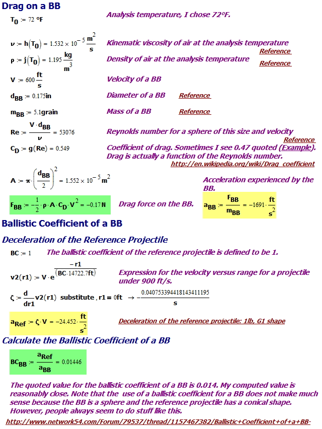
I received an email this weekend from a dad struggling to help his son with a project involving aerodynamic drag and BB gun. I did some quick calculations which I document here. I will try to look at pellets tomorrow. I was able to use basic principles to duplicate the empirical results quoted by manufacturers.
I will be computing three numbers associated with an air rifle shooting a BB:
The force of drag on the BB as it leaves the muzzle
The deceleration of the BB as it leaves the muzzle
The Ballistic Coefficient (BC) of a body is a measure of its ability to overcome air resistance in flight. It is inversely proportional to the negative acceleration — a high number indicates a low negative acceleration.
A projectile with a small deceleration due to atmospheric drag has a large BC. Projectiles with a large BC are less affected by drag and have performance closer to their performance in a vacuum.
While the Wikipedia definition is accurate as far as it goes, it does not allow you to compute the BC of a projectile. Equation 1 shows you how to compute the BC of any projectile.
Eq. 1
where
aReferenceProjectile is the acceleration of a reference projectile (eg. G7).
aProjectile is the acceleration of the projectile we are interested in.
Coefficient of Drag Given Reynolds Number
Figure 1 shows the coefficient of drag graph that I digitized using Dagra for this example.
Figure 1: Coefficient of Drag Versus Reynolds Number.
Density and Viscosity Data for Interpolation
Figure 2 shows the table from this web site that I interpolated so that I could get the density and viscosity of air at various temperatures.
Figure 2: Air Density and Viscosity Data.
Analysis
Interpolation of the Air Data
Figure 3 shows how I used Mathcad to interpolate all this data.
Figure 3: Digitization Code for Graphical Data.
Calculations
Figure 4 shows how I calculated the
force of drag on the BB
acceleration experienced by the BB
ballistic coefficient of the BB
Figure 4: Calculations for the Drag and Ballistic Coefficient of a BB.
Conclusion
I computed three numbers associated with an air rifle shooting a BB:
The force of drag on the BB as it leaves the muzzle: 0.17 N = 0.038 pound = 0.613 ounce
I cannot find corroborating information on the web. However, I use this number to compute the ballistic coefficient, for which I do find corroborating evidence.
The deceleration of the BB as it leaves the muzzle: 1691 ft/sec2
Straightforward application of Newton's second law.
The ballistic coefficient of the BB: 0.014
This agrees with data I have seen on forums here and here.
If you've been playing poker for half-an-hour and you don't know who the patsy is – your're the patsy.
— Warren Buffet
I love proofs without words. Usually, I see them in discussions of mathematical concepts like the Pythagorean theorem (examples). While reading about home construction at the Journal of Light Construction, I saw a nice graphical look at the difference between the gross margin on a product and the markup on a product.
If winning isn't everything, why do they keep score?
— Vince Lombardi
It is cold in Minnesota right now and I hear the local motorheads warning people not to run their gas tanks down to empty. During winter, I hear this warning because of concerns that water vapor in the gas tank may freeze and cause the vehicle to stop. I also hear concerns about running on a low fuel tank during the heat of summer because the fuel is need to cool the fuel pump, which is often mounted in the tank. Some folks also say that there is corrosion at the bottom of the gas tank that get sucked into the fuel pump when running the tank near empty.
The recommendation is usually that people should not let their tank go below quarter full. I don't know how serious these problems are, but they sound plausible. This rule means that you have to refuel more than someone who lets their gas tank go all the way to empty.
A software engineer who grew up on a farm commented that his father demanded that they fill their gas tanks when the tanks got down to 1/3 of a tank. His father was concerned that there could be an accident and someone may need to be rushed to the hospital. The nearest hospital was 1/3 of a full tank away. As I understand it, his father had heard of an accident where they could not get a child to the hospital in time to save him because a vehicle had been left on empty and they could not refuel it quickly enough. His father wanted to be sure that would not happen to his family. That seemed like a good reason to keep their gas tanks relatively full.
The need to fill your gas tank sometimes looms large in history. Once of the things that contributed to the demise of the battleship Bismarck (Fig. 1) was that it had not filled its fuel tanks when it had an opportunity. There were reasons not to fill her tanks, but in hindsight they were not good reasons.
Figure 1: Battleship Bismarck (Source: Wikipedia).
I remember reading that US Navy fighters providing air cover for aircraft carriers (Fig. 2) never let their fuel tanks run below 70% full. Their concern is readiness -- fighters burn a lot of full when they maneuver and they wanted to be sure to have plenty of fuel in the event they need to engage a foe on short notice. This means that they need to refuel very often. They takeoff with just enough fuel to get them to a tanker aircraft -- they literally refuel right after takeoff. Reducing the weight of fuel means that they can takeoff with a larger weapons load. They then have to refuel times more often than if they run their tanks down to empty.
Figure 2: Fighters Flying Top Cover Over the Aircraft Carrier Kitty Hawk.
It seems like you should refuel based on the cost of needing to refuel at a bad time. If you cannot afford to refuel during an emergency, you need to keep your tank relatively full at all times. The price you pay is more frequent refueling.
I write a lot of programs and I can't claim to be typical but I can claim that I get a lot of them working for a large variety of things and I would find it harder if I had to spend all my time learning how to use somebody else's routines. It's much easier for me to learn a few basic concepts and then reuse code by text-editing the code that previously worked.
- Donald Knuth
Introduction
Figure 1: Tobacco is slightly radioactive. (Source)
I have been reading about the safety hazards associated with traveling to Mars. One of the hazards is radiation. Since I know very little about the biological hazards associated with radiation, I have some learning to do. One of the ways I learn about a subject is to work through problems from the various online and library references that are available. During my investigation, I came across four excellent articles on the subject of radiation exposure from smoking tobacco. So, if being unlikely to get a decent life insurance policy wasn't enough to keep you from giving up tobacco then hopefully this revelation will do the trick! This simple example illustrates the basic calculation process.
I will summarize the information here using a Fermi-type of analysis. As noted in the comments section, estimating the absorbed dose from the radiation activity level is never easy. My work here is very approximate, but does produce results in the same range as stated by the US National Institutes of Health. My overall objective is to build some tools to help me understand the effects that radiation in space and on Mars have on people.
Background
Reference Articles
My post was motivated by the following information I encountered on the web:
The EPA addresses the source of the radiation from tobacco:
Naturally-occurring radioactive minerals accumulate on the sticky surfaces of tobacco leaves as the plant grows, and these minerals remain on the leaves throughout the manufacturing process. Additionally, the use of the phosphate fertilizer Apatite – which contains radium-226, lead-210, and polonium-210 – also increases the amount of radiation in tobacco plants.
The radium-226 that accumulates on the tobacco leaves predominantly emits alpha and gamma radiation. The lead-210 and polonium-210 particles lodge in the smoker's lungs, where they accumulate for decades (lead-210 has a half-life of 22.3 years). The tar from tobacco builds up on the bronchioles and traps even more of these particles. Over time, these particles can damage the lungs and lead to lung cancer.
Figure 2 provides an excellent illustration of how polonium-210 (210Po), uranium-238 (238U), and lead-210 (210Pb) get into tobacco (Source: Mel Porter).
Figure 2: How Polonium Get Into Tobacco.
Appendix A goes into detail on how 210Po actually gets into the leaves because of 222Rn.
I found a number of quite different values quoted for the radiation level of tobacco leaves. I decided to choose the value that reflected the average radioactivity levels for US tobacco. US tobacco is more radioactive than others, possibly because of our use of slightly more radioactive fertilizers.
Energy absorbed by a kg of a substance. The absorbed dose is represented symbolically by DT,R, with T representing the specific tissue (e.g. brain) and R representing the specific type of radiation (e.g. x-ray). Absorbed dose is measured in units of Gray (Gy). By definition, 1 Gy = 1 joule/kg.
Equivalent dose is the absorbed dose weighted by the effect of the different types of radiation. The equivalent dose is represented symbolically by HT and computed by the formula , where wR represents the weighting for radiation effects relative to x-rays (wX-Rays=1). Equivalent dose is measured in units of Sieverts (Sv).
Effective dose is the equivalent dose weighted by the radiation sensitivities of the different tissues. The effective dose is represented symbolically by E and computed by the formula , where wT represents the weighting for tissue radiation sensitivity. The tissue radiation sensitivity is normalized so that weights for all tissues sum to 1. Effective dose is measured in units of Sieverts (Sv).
Radiation Units
Sievert
The Wikipedia defines the Sievert (symbol: Sv) as the SI derived unit of equivalent radiation dose. The Sievert represents a measure of the biological effect, and should not be used to express the unmodified absorbed dose of radiation energy, which is a physical quantity measured in Grays.
Gray
The Gray (symbol: Gy) is the SI derived unit of absorbed dose. Such energies are typically associated with ionizing radiation such as X-rays or gamma particles or with other nuclear particles. It is defined as the absorption of one joule of such energy by one kilogram of matter.
Analysis
My calculations use the same approach as David Gillies in his forum posting. However, my inputs ended up being different and I obtained a different result.
Discussion of Steady State Radiation Level
Over time, the radiation level emitted from cigarette smoking approaches a steady-state level. The steady state level is reached when the 210Po that decays each day is exactly cancelled by the amount of 210Po that is being inhaled every day. My analysis assumes that the smoker has reached steady state.
Definition of Units
Figure 3 shows the various units that I defined for this problem solution.
Figure 3: Units Defined for My Analysis.
Weighting of Effects By Radiation Type
Figure 4 shows the biological weighting factors for different kinds of radation. 210Po emits alpha particles, which have a weighting factor of 20 relative to x-rays.
Figure 4: Weighting of the Different Radiation Types.
Polonium Characteristics
Figure 5 shows the relevant facts on 210Po.
Figure 5: Characteristics of Polonium-210.
Radiation Model
Figure 6 shows my calculations for the effective radiation dose that a 1.5 pack a day smoker endures.
Figure 6: Radiation Calculations for 1.5 Pack a Day Smoker.
Conclusion
I was looking for a simple example of computing the effects of radiation on a human. This example produces a result that is consistent with the data in the Wikipedia.
Appendix A: Source of Polonium
210Po is generated as a decay product from 222Rn. Here is the decay chain for 222Rn, which has 210Po as an intermediate product (Source). I highlighted the isotopes mentioned above.
222Rn, 3.8 days, alpha decaying to...
218Po, 3.10 minutes, alpha decaying to...
214Pb, 26.8 minutes, beta decaying to...
214Bi, 19.9 minutes, beta decaying to...
214Po, 0.1643 ms, alpha decaying to...
210Pb, which has a much longer half-life of 22.3 years, beta decaying to...
All content provided on the mathscinotes.com blog is for informational purposes only. The owner of this blog makes no representations as to the accuracy or completeness of any information on this site or found by following any link on this site.
The owner of mathscinotes.com will not be liable for any errors or omissions in this information nor for the availability of this information. The owner will not be liable for any losses, injuries, or damages from the display or use of this information.


 .
.


 , where wR represents the weighting for radiation effects relative to x-rays (wX-Rays=1). Equivalent dose is measured in units of Sieverts (Sv).
 , where wT represents the weighting for tissue radiation sensitivity. The tissue radiation sensitivity is normalized so that weights for all tissues sum to 1. Effective dose is measured in units of Sieverts (Sv).


