Quote of the Day
The odds are good, but the goods are odd.
— Statement made by an Alaskan woman after she told me that there were 1.6 men for every woman in her town.
Introduction

Figure 1: Power Lines are Hazardous for Low-Flying Airplanes.
I was reading an article in Photonics Spectra magazine about the use of a laser radar system to assist pilots in detecting wires while flying low (Figure 1), and I saw two commonly used bandwidth estimation formulas that most engineers do not think much about. I have worked on laser radar systems in my past and the bandwidth of these systems drives their cost and performance. I thought it would be useful to review how engineers estimate the bandwidth required for the pulse detection circuits used in these systems.
I should point out that electrical circuits process signals that vary in time, but these circuits are usually designed based on the frequency content of the signals being processed. A co-worker once told me that
Electronic systems are hard to design using time-based approaches (e.g. differential equations), but are relatively easy to design using frequency-based approaches (e.g. Bode plots). Unfortunately, it is relatively hard to test electronic systems using frequency-based approaches, but these same systems are usually easy to test using time-based methods (e.g. oscilloscopes). Thus, we need to become proficient at switching between both time and frequency points of view.
I have found this bit of wisdom to often be true.
Background
Why do we care about bandwidth?
The bandwidth of a circuit tells us the range of signals that the circuit must process in order to meet the performance requirements of the system. Unfortunately, narrowband problems are easier and cheaper to solve than wideband problems.
Definitions
The words "narrow" and "wide" are relative terms. Thus, the definitions of narrowband and wideband are relative terms as well.
- Narrowband
- A narrowband circuit is a circuit that can process the signals through it as if were a single frequency.
- Wideband
- A wideband circuit is a circuit that must process a range of frequencies that cannot be treated as if they were a single frequency.
My Objective
In practice, all real signals have infinite bandwidth. Because real circuit cannot process infinite bandwidth signals, we need to approximate infinite bandwidth signals with finite bandwidth signals. In general, wider bandwidth implies a greater percentage of the signal energy or power being processed by the circuit. For the discussion that follows, I will be working with energy because a pulse has finite energy and this radar detects pulses. The same type of analysis holds for random pulse sequences or continuous waveforms, which have a finite power level. You use power for signals that exist for long times (theoretically, infinitely long) and energy for signals that exist for finite times.
There are two common bandwidth approximations used in electrical engineering.

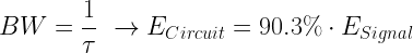
where
- ESignal is the total energy in a pulse.
- ECircuit is the total pulse energy processed by the circuit.
- τ is the pulse width.
- BW is the circuit bandwidth.
Analysis
I will approach the problem in two stages:
- Derive the Fourier Transform of a Pulse Signal
This is a direct application of the Fourier Transform to a normalized pulse waveform (unit width and height).
- Derive a Formula for the Percentage of Signal Energy As a Function of Bandwidth
Higher fidelity systems process a higher percentage of the total signal energy. I will derive an expression for the signal energy percentage as a function of circuit bandwidth and will plot it.
Derivation
Figure 2 shows my derivation of the Fourier transform of a unit pulse.

Figure 2: Definition of the Fourier Transform of a Pulse.
Energy Percentage Versus Bandwidth
Figure 3 shows my derivation of a formula for the percentage of signal energy as a function of bandwidth.
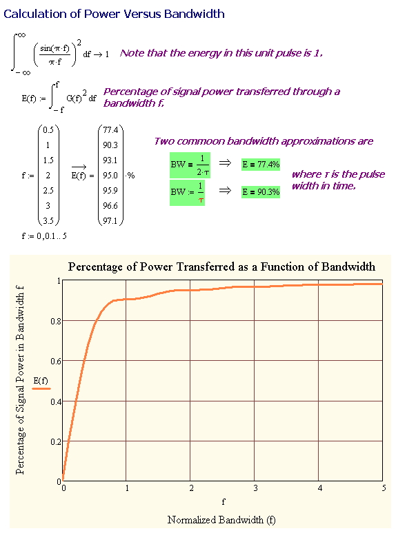
Figure 3: Energy Versus Bandwidth
Conclusion
While reading the article mentioned in the introduction, I started to wonder what fraction of the signal energy was being processed by the circuit. I could not remember the energy fractions, so I decided to re-derive them here.


 , where m is the mass of the animal in question.


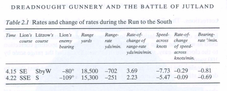
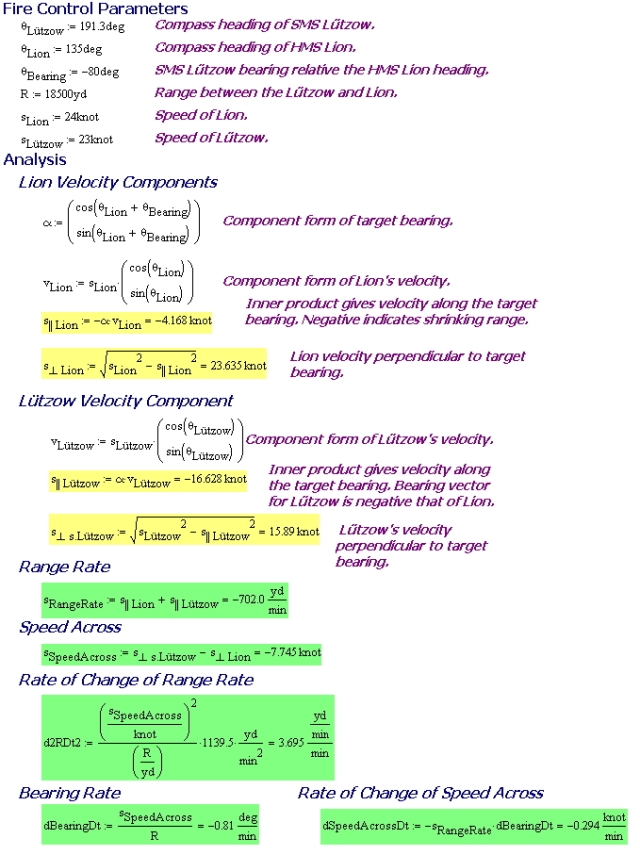
 : Range Rate of Change
 : Target Bearing Rate of Change
 : Rate of Change of the Range Rate