Fire Control Formulas from World War 1

Quote of the Day

When fascism comes to America, it will be wrapped in the flag carrying the Cross.

— Sinclair Lewis


Introduction

Figure 1: HMS Dreadnought, the ship that changed the direction of naval gunnery.

Figure 1: HMS Dreadnought, the ship that changed the direction of naval gunnery. (Source)

I am reading the book "Dreadnought Gunnery and the Battle of Jutland: The Question of Fire Control". This very informative book provides the details on how fire control developed during its very early days. This period of time is interesting to me because, in my opinion, it was the start of modern computing. The big naval revolution driving the development of fire control was the introduction of long-range torpedoes (see Whitehead Torpedo). Prior to the arrival of torpedoes, ships simply engaged at ranges that allowed them to directly point their guns at one another, a process referred to as direct fire. The threat from torpedoes drove ships to engage at longer ranges that required the development of indirect fire. Indirect fire means aiming and firing a projectile without relying on a direct line of sight between the gun and its target. Effective indirect fire meant developing a number of new technologies: range finding, precision hydraulics, control systems, and calculation systems.

A Google Preview of "Dreadnought Gunnery" is available here if you are curious about the book. I have read some criticism of the book on Amazon because it is a slightly reworked PhD thesis. That doesn't bother me in the least, but some folks may not like the academic writing style. The book's Appendix contains a one-page summary of the fire control formulas that were solved by the analog computers used on the Dreadnoughts (Figure 1). The equations seemed a bit odd to me until I derived them myself. It turns out I have seen them before, but in a different form. I thought I would show the equivalences here. I will be using these fire control formulas in some simulations I plan to prepare. Ultimately, I want to do some analysis of the error sensitivity of these formulas.

All the mathematics is in this post is done in Mathcad. I use Mathcad's unit handling ability to perform the various conversions required.

Background

Figure 2 is a scan of the fire control formulas shown in the Appendix of "Dreadnought Gunnery". I have added some markups in tan to indicate my names for the various equations.

Figure 1: Fire Control Equations from "Dreadnought Gunnery".

Figure 2: Fire Control Equations from "Dreadnought Gunnery".

I will derive these formulas and show how they are similar to formulas you have seen in other contexts.

Analysis

Mathematical Objectives

Battleship gunnery used mechanical integrators to convert measured range and bearing rates into projected target positions in the future. These projections are important because projectiles require time to arrive at their target location -- a concept referred to as deflection or lead (rhymes with "need"). The Appendix in "Dreadnought Gunnery" derives three rate expressions.

  • \frac{dR}{dt}: Range Rate of Change
  • \frac{d\beta }{dt}: Target Bearing Rate of Change
  • \frac{{{d}^{2}}R}{d{{t}^{2}}}: Rate of Change of the Range Rate

These are the formulas that I will focus on. They are presented in the Appendix using units of knots, yards, degrees, and minutes. This will introduce some conversion constants.

Own Ship and Enemy Fire Control Geometry

One of the things that confuses me about the formulas in Figure 1 is their notation. For example, x is used to represent the relative velocity of the enemy ship in a direction perpendicular to the range vector. I prefer to call this velocity component vp. The variable a is used to represent the relative velocity of the enemy ship in the direction of the range vector. I prefer to call this velocity component vr. I REALLY like variable names that mean something to me (e.g. v for velocity). I also changed designation of the target angle relative to the range vector from an iota (ι) to a theta (θ) because it is easier to see a theta. So I renamed all the variables in Figure 2 to what you see in Figure 3.

Figure 2: Updated Fire Control Geometry.

Figure 3: Updated Fire Control Geometry.

Range Rate Formula

The range rate equation is simply the relative radial velocity between the own ship and the enemy ship. This calculation involves a little bit of vector math and then some unit conversions, which are shown in Figure 4.

Figure 3: Derivation of Range Rate Equation.

Figure 4: Derivation of Range Rate Equation.

Note that in Figure 4 I show the variables ves and vos divided by knot. This approach is used in Mathcad to perform unit conversion.

Bearing Rate Formula

Figure 5 shows my derivation of the bearing rate formula. Note that the Appendix refers to a magnetic bearing and in Figure 2 I show a line-of-sight bearing (i.e. bearing relative to a ship's course). If the ship is not changing course, the rate of change in magnetic bearing and the rate of change in line-of-sight bearing are equal. I make this assumption in Figure 5.

Figure 4: Derivation of Bearing Rate Formula.

Figure 5: Derivation of Bearing Rate Formula.

This equation is really a restatement of the angular velocity equation from elementary physics.

Rate of Change of the Range Rate

Figure 6 shows my derivation of the rate of change of the range rate.

Figure 5: Rate of Change of Range Rate Derivation.

Figure 6: Rate of Change of Range Rate Derivation.

The rate of change of the range rate is really just a restatement of the centripetal acceleration equation from elementary physics.

Conclusion

I was able to derive all the expressions from the Appendix of "Dreadnought Gunner". I was also able to show the expressions in the Appendix are actually commonly seen equations from physics, just hidden a tad by notation.

Posted in Ballistics, History of Science and Technology, Military History | 11 Comments

WW2 Sub Skippers Were Very Young

Quote of the Day

I am not a product of my circumstances. I am a product of my decisions.

— Stephen Covey


I was watching this Youtube video about two famous WW2 submarine skippers, Morton and O'Kane, and I started to wonder just how old these skippers were during WW2.

Hollywood movies usually show WW2 sub skippers as men in their late 40s or 50s (e.g. Operation Pacific or Run Silent Run Deep). I found a list of the top scoring US submarine skippers of WW2 and was able to figure out their birthdays. Given their birthdays, I determined that they had an average age of 32 years on December 7th, 1941.  The following table summarizes their ages and their post-war "ships sunk" scoring. When you think about the responsibility they had, these men were very young.

Ships Sunk Rank Captain Birthday Age at time of Pearl Harbor Attack Ships Sunk Tonnage
1 Richard H. O'Kane 02-Feb-1911 30 Years, 10 Months and 5 Days 24.0 93,824
2 Slade D. Cutter 01-Nov-1911 30 Years, 1 Months and 6 Days 19.0 71,729
3 Dudley W. Morton 17-Jul-1907 34 Years, 4 Months and 20 Days 19.0 54,683
4 Eugene B. Fluckey 05-Oct-1913 28 Years, 2 Months and 2 Days 16.3 95,360
5 Samuel D. Dealey 13-Sep-1906 35 Years, 2 Months and 24 Days 16.0 54,002
6 Reuben T. Whitaker 23-Sep-1911 30 Years, 2 Months and 14 Days 14.5 60,846
7 Gordon W. Underwood 03-Jun-1910 31 Years, 6 Months and 4 Days 14.0 75,386
8 Royce L. Gross 29-Sep-1906 35 Years, 2 Months and 8 Days 14.0 65,736
9 Charles O. Triebel 17-Nov-1907 34 Years, 0 Months and 20 Days 14.0 58,837
10 John S. Coye Jr. 24-Apr-1911 30 Years, 7 Months and 13 Days 14.0 38,659
11 William B. Sieglaff 06-Jul-1908 33 Years, 5 Months and 1 Days 13.0 32,886
12 Thomas S. Baskett 04-Sep-1913 28 Years, 3 Months and 3 Days 12.0 27,273
13 Henry C. Bruton 15-Feb-1905 36 Years, 9 Months and 22 Days 11.0 54,564
14 Bafford E. Lewellen 22-Sep-1909 32 Years, 2 Months and 15 Days 11.0 23,685
15 Charles H. Andrews 14-May-1908 33 Years, 6 Months and 23 Days 10.0 57,243
16 Robert E. Dornin 30-Dec-1912 28 Years, 11 Months and 7 Days 10.0 54,595
17 Eric L. Barr Jr. 02-May-1912 29 Years, 7 Months and 5 Days 10.0 46,212
18 Ralph M. Metcalf 22-Jun-1913 28 Years, 5 Months and 15 Days 10.0 40,040
19 Raymond H. Bass 15-Jan-1910 31 Years, 10 Months and 22 Days 10.0 37,977
20 Malcolm E. Garrison 29-Mar-1910 31 Years, 8 Months and 8 Days 10.0 37,368
21 Thomas B. Klakring 19-Dec-1904 36 Years, 11 Months and 18 Days 10.0 33,122
22 John A. Moore 12-Jan-1910 31 Years, 10 Months and 25 Days 9.5 45,757
23 Glynn R. Donaho 25-Mar-1905 36 Years, 8 Months and 12 Days 9.5 29,870
24 Eli T. Reich 20-Mar-1913 28 Years, 8 Months and 17 Days 9.0 59,839
25 Walter T. Griffith 03-Jun-1911 30 Years, 6 Months and 4 Days 9.0 45,874
  Average Age   32 Years, 0 Months and 0 Days   1,295,367

Note that in 1940 (pre-WW2), the average age of an Army major (comparable to Navy Lt. Commander) was 48. The demands of war thrust young people into command roles much more quickly than in peacetime.

Posted in History Through Spreadsheets, Military History | 3 Comments

Inserting Images into Excel Comments Using VBA

I use Excel for basic statistical analysis of manufacturing and field return data as part of daily routine. I also use Excel for department budgeting. During these tasks, I frequently need to add information to my spreadsheets about my information sources (see Wikipedia entry on data provenance). Since much of my information comes to me in the form of email or web pages, a quick and easy way to document this information is to take a screenshot of the information and insert the information into an Excel comment.

For years I have included images in Excel comments using the manual procedure described here. This approach works well but is slow. I finally decided that there has to be a better way and I wrote a Visual Basic for Applications (VBA) macro that handles all the ugly details. Here is a link to this spreadsheet. The spreadsheet does use a VBA macro. If you are concerned about security, just look in the macro and see what it does.

To see a sample image (Saturn), just mouse over the cell with the little red triangle in the upper right corner.

A little discussion on how to use the macro is in order:

  • Put an image into your clipboard (I use PicPick)
  • Select the cell where you want to put the image
  • Click the button labeled "Press"
  • Your selected cell will now have little red triangle in the upper right corner. You will see your image when you mouse over this cell.
  • I used a button for this example, but in my work I assign both a Quick Access toolbar icon and a keyboard shortcut to this macro.

Many thanks to the folks at these two web sites for posting code and clues that helped me put this macro together.

Posted in Management, software | 27 Comments

A Tale of Getting Older

I was with a couple I have known for years this weekend. They have two daughters separated in age by five years. The younger daughter is just finishing high school and still lives at home. The older daughter is no longer living at home, but was visiting her parents this weekend. The tale begins with the daughters in the kitchen hearing their parents having the following dysfunctional discussion.

Father from the kitchen:  ”I can’t find my glasses – do you know where my glasses are?”

Mother from upstairs: ”Molasses? It’s in the cupboard.”

Father from kitchen: ”Not molasses, glasses ..”

The mother and father went back and forth like this for a while. It was a classic case of two people not quite hearing things correctly. The two young women listened quietly to this miss-communication. After the mom and dad got things straightened out, the younger daughter turned to her older sister and said, “At least you had them during their good years.”

Her response was priceless.

Posted in Personal | Tagged | Comments Off on A Tale of Getting Older

Another Glamour Shot from the World of Engineering

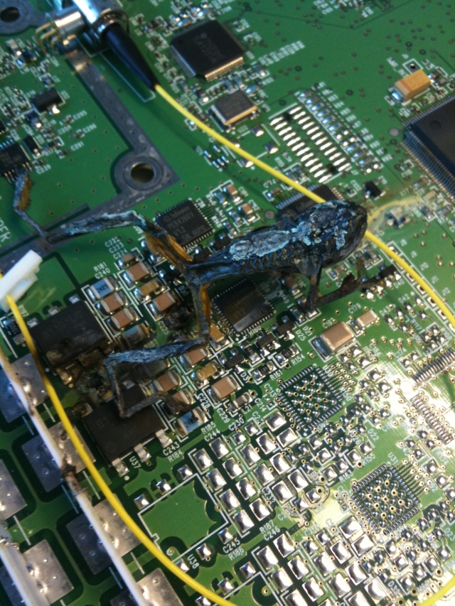
Things are starting to get cold now in Minnesota and all nature's creatures are looking for a nice warm place to stay for the winter -- including me. Today's photo shows a frog who found one of my optical network terminals a nice, warm place to hang out. Unfortunately, he decided to place himself right on top our our phone ringer circuit. This circuit generates over 100 V when ringing a phone. Apparently, someone called this customer after the frog had positioned himself on top of the ringer circuit. Frogs do not do well with 105 V placed across their little bodies.
frog

Posted in Electronics | Comments Off on Another Glamour Shot from the World of Engineering

More Bugs in My Optics

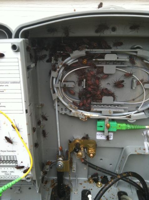
I had another optical failure related to bug intrusion. I do not yet understand how the bugs do it, but somehow they increase my optical loss enormously. This particular optical node was not properly sealed and box elder bugs got in. They are looking for a warm place to winter. Figure 1 shows what it looked like in the field. My wife does not like these bugs at all -- I will not show her this photo.

Figure 1: Box Elder Bugs Inside an Optical Network Unit.

Figure 1: Box Elder Bugs Inside an Optical Network Unit.


While people may think an engineer's work is always high tech, I want to remind them that we spend a lot of time on little things -- like making sure bugs and water cannot ruin our day. Still, it would be nice if we could find a way to get rid of these horrible things once and for all from locations like this. Having the node sealed is one way to keep them out, but some bugs (like termites) can chew through the casing and worm inside regardless, which can be an absolute nightmare. I know some services exist to help keep these issues down, like the terminix pest control options on the market, so perhaps next time I will give those a go.

It really is something else to open a case expecting to deal with a burnt-out wire or some technical difficulty only to have to scrape so many bugs away instead. Hardly a sanitary thing to experience, truth be told.

Posted in Fiber Optics | Comments Off on More Bugs in My Optics

Example of a Useful Histogram

Sometimes all it takes is to use a histogram maker to create a graph, for example, to help provide you the clue you need to solve a mystery. Currently, I am working on reducing the failure rate of Avalanche Photo-Diodes (APDs). I found a histogram was useful in my work and I thought I would share it.

APDs are sensitive light detectors. In fact, some can detect individual photons. In my case, APDs are a critical component in the receiver circuit of an optical network. To achieve maximum sensitivity, APDs require a specific voltage be placed across them, which we call the bias voltage. We determine this voltage for each APD during manufacturing through a process we call calibration. The calibration process uses a steepest descent algorithm to the determine the bias voltage that provides maximum sensitivity.

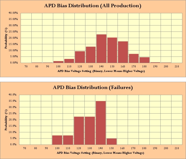
My APD failure rate is too high (still less than 1%) and I need to find out why. I was not making much progress, but then I decided to generate a histogram of APD bias voltages of the failed units and of the general population of APDs we have shipped. This histogram is shown below.

Figure 1: Histograms of APD Bias Voltage for All Units and Failures.

Figure 1: Histograms of APD Bias Voltage for All Units and Failures.


You can see in Figure 1 that the failed units have APD bias voltages that are in the high range of the overall population (high voltage implies low binary setting). I shared this figure with a co-worker and we began discussing why this could be the case. Within a few minutes, we had a number of potential failure causes to check out. I now believe we are on our way to solving our mystery.

I often find myself looking for patterns and regularities in data. Graphs are one of the key techniques we use to see these patterns. In this respect, I do find myself drawn to the work of Tufte. I don't agree with everything he says, but there is a lot of material there that makes me think.

Posted in Electronics | Comments Off on Example of a Useful Histogram

Candle Flame in Space

Quote of the Day

Only enemies speak the truth. Friends and lovers lie endlessly, caught in the web of duty.

— Stephen King


I saw this photo posted by Robert Frost here. It shows a flame on Earth (left) and a flame in space (right). Very cool ...
Candle Flame in Space

Posted in Astronomy, General Science | Tagged | Comments Off on Candle Flame in Space

World War 2 Industrial Casualties

Quote of the Day

Solomon had 300 wives and 700 porcupines.

- Kevin Kling, quoting a little boy in a religion class describing Solomon.


Introduction

Figure 1: Poster Encouraging Job Safety.

Figure 1: Poster Encouraging Job Safety (Source).

I like to watch authors discuss their history books on BookTV. I listen to BookTV while I work around the house. One weekend, I heard two historians (I did not write down their names) discussing World War 2 and each mentioned a statistic that sounded something like this (my wording).

During World War 2, the US took the better part of 18 months to build its military-industrial base after Pearl Harbor. Building this industrial base had its own cost in lives. In fact, the number of US military personnel killed in action each year did not exceed the number of US industrial deaths each year until sometime in 1943.

I had never considered the number of people that were dying on the home-front building the armaments needed to fight World War 2. I thought that I should be able to fact check this statement – work that I document in this post.

Background

I did a quick web search and found the following sources.

  • This post consists of grabbing this data, cleaning it up, and summarizing the results in a pivot table.

    If you want to see how I processed the data, here is my spreadsheet.

    Analysis

    The historians were correct if you strictly take casualties listed as Killed in Action (KIA) or air combat deaths. To keep things simple, I focused on the data for the US Army, Navy, and Marines – I could not find yearly Coast Guard data, but did find yearly Merchant Marine data (shown in the attached spreadsheet). I grabbed all the KIA data on the pages listed above and generated a pivot table (Table 1), which I show below. The casualties in war are never-ending and it can be jarring to see on paper. People want to show their support for those who serve by honoring their memory, whether that be flying marine corp flags outside their homes to attending the ceremonies that happen throughout the year. All we can say is that those KIA are never forgotten, on paper or in the mind. One could never know how big their sacrifice is and they will always be remembered by the country and their loved ones (through Toledo Blade obituaries or similar others), for their valour and conviction.

    It was during 1943 that the number of military KIA exceeded the number of workers dying in factories. The table also shows that military casualties really surged during 1944, which makes sense when you think of D-Day and the increasing tempo of operations in the Pacific War. Note that the official records list some deaths as occurring in 1946. I have included these deaths in 1945, which is why I label 1945 with a plus.

    Table 1: US Army, Navy, and Marine World War 2 Killed in Action Statistics.

    Year

    Army

    Marines

    Navy

    Military KIA

    Factory Deaths

    1941

    467

    99

    2,181

    2,747

    18,000

    1942

    4,497

    1,239

    2,890

    8,626

    18,500

    1943

    19,548

    1,732

    4,839

    26,119

    17,500

    1944

    107,437

    5,892

    8,187

    121,516

    16,000

    1945+

    57,747

    8,414

    15,907

    78,678

    16,000

    Totals

    189,696

    17,376

    34,004

    237,686

    85,500

    I would argue that these numbers are not really fair because there are many other battle deaths not listed as KIA. I get Table 2 if I count all the battle and non-battle-related deaths, and you can see the military deaths swamp out the civilian deaths in 1942.

    Table 2: US Army, Navy, and Marine World War 2 Battle and Non-Battle Killed Statistics.

    Year

    Army

    Marines

    Navy

    Military KIA

    Factory Deaths

    1941

    493

    165

    2,217

    2,875

    18,000

    1942

    17,612

    1,607

    3,278

    22,497

    18,500

    1943

    22,592

    1,839

    5,251

    29,682

    17,500

    1944

    126,170

    5,746

    9,348

    141,264

    16,000

    1945+

    68,007

    10,376

    16,856

    95,239

    16,000

    Totals

    234,874

    19,733

    36,950

    291,557

    85,500

    These totals agree with those reported by the Wikipedia. For total Army, Navy, and Marine casualties, see Appendix B.

    The US Marine's listed their casualties by battle and not by year. I obtained the list of US Marine casualties by year from a book quote on a forum post (see Appendix A).

    Conclusions

    Here is what I learned from this data:

    • US factory work in the early 20th century was dangerous.
      • For comparison, there were 4,679 fatal work injuries in the US during 2014.
      • There were ~149 million employed workers in the US during 2015. (Source)
      • There were ~53 million employed workers in the US during 1945. (Source)
      • Roughly, there was more than 3 times the number of fatal work injuries with a workforce ~1/3 the size.
    • 48% of all US military KIA occurred during 1944.
      • The number of KIA in 1945 was lower than in 1944 because most of the fighting ended by June 1945.
      • 1945 casualty rates dropped enormously after the Battle of Okinawa and VE day.
    • The size of the European theater was massive compared to the Pacific theater.
      • Just look at the US Army casualties after D-Day. The US Army in July 1944 had 16.8K soldiers killed, where the US Marines lost 19.7k for the entire war.

    Appendix A: US Marine Casualties By Year

    I was able to find a forum post that summarized the Marines casualties by year using data from the book The US Marine Corps Story (ISBN 0316585580). Table 3 summarizes this information.

    Table 3: Marine World War 2 Killed in Action Statistics.

    Year

    Killed

    Wounded

    Captured

    Missing

    Total Casualties

    1941

    165

    80

    740

    0

    985

    1942

    1,607

    3,336

    1,292

    85

    6,320

    1943

    1,839

    4,996

    0

    27

    6,682

    1944

    5,746

    21,078

    0

    117

    26,941

    1945+

    10,376

    37,717

    238

    0

    48,331

    Totals

    19,733

    67,207

    2,270

    229

    89,439

    Appendix B: Battle and Non-Battle Casualties

    Table 4 shows the total Army, Navy, and Marines casualties during WW2 (Source). Note that there were a significant number of non-battle related casualties. This is true in all conflicts.

    Table 4: US Army, Navy, and Marines WW2 Casualty Summary.
    Service Total Serving Battle Deaths Non-Battle Deaths Total Deaths Wounded
    Army 11,260,000 234,874 83,400 318,274 565,861
    Navy 4,183,466 36,950 25,664 62,614 37,778
    Marines 669,100 19,733 4,778 24,511 67,207
    Totals 16,112,566 291,557 113,842 405,399 670,846

    Appendix C: Industrial Casualty Table.

    Figure 2 is my screen capture of the government's data on factory deaths (Source).

    Figure M: Screen Capture From Google Books on Industrial Casualties.

    Figure 2: Screen Capture From Google Books on Industrial Casualties.

    Appendix D: Alternate Industrial Casualty Reference.

    Figure 3 is my screen capture from The Cambridge History of the Second World War: Volume 3, Total War: Economy, Society and Culture (Link). The data in this post is consistent with this reference.

    Figure 3: Alternate Reference on Industrial Casualties.

    Figure 3: Alternate Reference on Industrial Casualties.

Posted in History of Science and Technology, History Through Spreadsheets, Military History | 24 Comments

Another Interpretation of the Ballistic Coefficient

Introduction

I love to look for physical interpretations of various constants. Sometimes it is impossible to come up with an interpretation, but such is not the case for the ballistic coefficient. This morning I read a very solid piece of technical work on the ballistic coefficient that has another interpretation that I have not seen before (Source). Here is a statement they made that I will support with a quick derivation.

To a rough approximation, the BC [ballistic coefficient] can be estimated as the fraction of 1000 yards over which a projectile loses half of its initial kinetic energy. In other words, a bullet with a BC of 0.300 should lose roughly half of its initial kinetic energy at a range of 300 yards.

This statement is very interesting in a number of ways:

  • Can I derive it using the expressions from Pejsa's book "Modern Practical Ballistics"?
  • What do they mean by "rough approximation"?
  • Does this approximation work with bullets that have a ballistic coefficient greater than 1?

I will address all three questions in this post. Let's dig in ...

Background

The ballistic coefficient is a very old school concept -- the ballistic coefficient is the ratio of a projectile's deceleration due to drag compared to the deceleration due to drag for a reference projectile of the same shape. Modern projectile simulation software would use different approaches (see McCoy). For my purposes here, we will define the ballistic coefficient C as shown in Equation 1.

Eq. 1 C\triangleq \frac{{{a}_{\text{Ref}}}}{{{a}_{\text{Projectile}}}}

where

  • aRef is the deceleration of a reference projectile.
  • aProjectile is the deceleration of our projectile under test.

Analysis

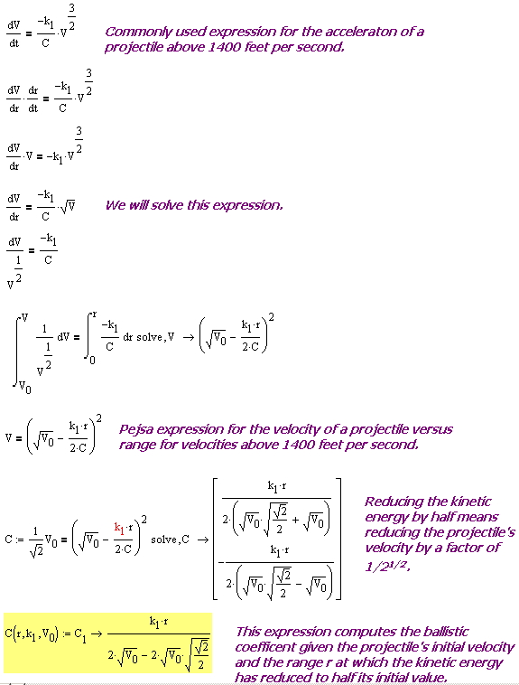
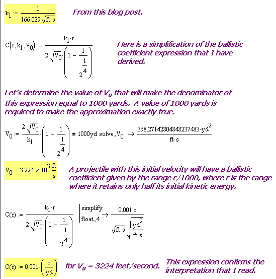
Figure 1 shows my derivation of an expression for the ballistic coefficient as a function of projectile velocity and range. The derivation presumes that reducing the kinetic energy by a factor of 2 means a velocity reduction by the \sqrt{2}.

Figure 1: Derivation of an Expression for the Ballistic Coefficient.

Figure 1: Derivation of an Expression for the Ballistic Coefficient.

Figure 2 complete my confirmation of the approximation. The approximation is exactly true for projectiles with an initial velocity of 3224 feet per second. It is approximately true for initial velocities near 3224 feet per second, which is common for high-velocity rifle projectiles.

Figure 2: Verification of the Approximation.

Figure 2: Verification of the Approximation.

Conclusion

Let's review my answers to the questions I presented in my Introduction.

  • Can I derive it using the expressions from Pejsa's book "Modern Practical Ballistics"?

    See Figure 2.

  • What do they mean by "rough approximation"?

    It is only exactly true for projectiles with an initial velocity of 3224 feet per second. It is only roughly true for initial projectile velocities near 3224 feet per second.

  • Does this approximation work with bullets that have a ballistic coefficient greater than 1?

    It is not too bad for a battleship projectile. Using the approximation and the range table here, I get that the 16 inch ballistic coefficient is ~13 (actual value of ~15). Not too bad considering the initial velocity is 2577 feet per second instead of 3224 feet per second.

Posted in Ballistics | 9 Comments