
Quote of the Day
Criticism may not be agreeable, but it is necessary. It fulfills the same function as pain in the human body. it calls attention to an unhealthy state of things.
— Winston Churchill
Introduction

Figure 1: Mk 13 HC (High Capacity) 16-inch Shells.
I received the following question on one of my earlier blog posts:
Naval guns claim a range of up to 16 miles, and apparently do so with an initial velocity of only approx. 3000 fps [, which is similar to rifle bullet]. how is this possible[?]
You can view my answer on that blog post, but I started to think about alternative, but equivalent, ways to answer this question. From a numerical standpoint, one way to answer his question is by comparing the ballistic coefficient of a 16-inch projectile (Figure 1) to that of a standard firearm projectile. A projectile with a large ballistic coefficient is less affected by drag than a projectile with a smaller ballistic coefficient. We can use the the ballistic coefficient to compare the effect of drag on different projectiles. A 16-inch projectile goes so much farther than a rifle bullet because the drag on the 16-inch projectile is relatively small compared to its momentum. Ultimately, this is because mass increases by the cube of the projectile dimensions and drag increases by the square of the projectile dimensions. This means that larger projectiles tend to have higher ballistic coefficients and drag has less effect.
Let's put some numbers together ...
Background
The Wikipedia defines the ballistic coefficient as follows:
- Ballistic Coefficient
- The Ballistic Coefficient (BC) of a body is a measure of its ability to overcome air resistance in flight. It is inversely proportional to the negative acceleration — a high number indicates a low negative acceleration.
A projectile with a small deceleration due to atmospheric drag has a large BC. Projectiles with a large BC are less affected by drag and have performance closer to their performance in a vacuum.
While the Wikipedia definition is accurate as far as it goes, it does not allow you to compute the BC of a projectile. Equation 1 shows you how to compute the BC of any projectile.
| Eq. 1 | 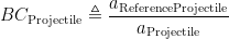 |
where
- aReferenceProjectile is the acceleration of a reference projectile (eg. G7).
- aProjectile is the acceleration of the projectile we are interested in.
Analysis
I will compute the BC of the US Navy's 16-in, high-capacity (1900 pound) shell that was fired by the Iowa-class battleships using a couple of different methods.
- Estimate the deceleration of the battleship projectile and compute Equation 1.
- Apply a geometry-based formula.
Both methods give similar answers.
Method Based on Deceleration Estimate
To estimate the 16-inch projectile's deceleration. There is data available for this. Figure 2 shows a snippet from a US Navy range table for the 16-inch projectile (Source).

Figure 2: Snippet from 16-inch Projectile Range Table (1900 lb).
For my BC estimate calculation (Figure 3), I will use only the forward velocity component because that component is experiencing the bulk of the drag.

Figure 3: Ballistic Coefficient Calculation Using Deceleration Data.
Ballistic Coefficient Calculation Using Formula
Figure 4 shows the ballistic coefficient calculation using a geometric formula that compares the 16-inch projectile to a 30-06 projectile (Ball, M2, 152 grain, 0.308 in diameter).

Figure 4: Computing the BC of a 16-inch Projectile Using a Formula.
Conclusion
Here is a quote that supports my analysis from "Modern Practical Ballistics" on page 115 (ISBN 0-96212776-3-7).
Modern long-range guns like the US Navy's 16-inch guns are able to attain ranges in excess of 25 miles using an initial elevation angle near 45 degrees; their shells reach an altitude of approximately seven miles. Although their muzzle velocities are generally only about 2600 to 2800 fps, their enormous size and weight -- in excess of 2000 pounds -- gives them ballistic coefficients of around 15, which are 30 to 50 times as great as small arms projectiles!


![\displaystyle d[\text{light-years }\!\!]\!\!\text{ =}\frac{{{d}_{AU}}[\text{km }\!\!]\!\!\text{ }}{\frac{\pi \left[ \text{radians} \right]}{180{}^\circ }\cdot \frac{\theta [\text{milliarcseconds }\!\!]\!\!\text{ }\cdot \text{0}\text{.001}\left[ \frac{\text{arcseconds}}{\text{milliarcseconds}} \right]}{3600\left[ \frac{\text{arcseconds}}{\text{degree}} \right]}\cdot {{d}_{LightYear}}[\text{km }\!\!]\!\!\text{ }}](https://s0.wp.com/latex.php?latex=%5Cdisplaystyle+d%5B%5Ctext%7Blight-years+%7D%5C%21%5C%21%5D%5C%21%5C%21%5Ctext%7B+%3D%7D%5Cfrac%7B%7B%7Bd%7D_%7BAU%7D%7D%5B%5Ctext%7Bkm+%7D%5C%21%5C%21%5D%5C%21%5C%21%5Ctext%7B+%7D%7D%7B%5Cfrac%7B%5Cpi+%5Cleft%5B+%5Ctext%7Bradians%7D+%5Cright%5D%7D%7B180%7B%7D%5E%5Ccirc+%7D%5Ccdot+%5Cfrac%7B%5Ctheta+%5B%5Ctext%7Bmilliarcseconds+%7D%5C%21%5C%21%5D%5C%21%5C%21%5Ctext%7B+%7D%5Ccdot+%5Ctext%7B0%7D%5Ctext%7B.001%7D%5Cleft%5B+%5Cfrac%7B%5Ctext%7Barcseconds%7D%7D%7B%5Ctext%7Bmilliarcseconds%7D%7D+%5Cright%5D%7D%7B3600%5Cleft%5B+%5Cfrac%7B%5Ctext%7Barcseconds%7D%7D%7B%5Ctext%7Bdegree%7D%7D+%5Cright%5D%7D%5Ccdot+%7B%7Bd%7D_%7BLightYear%7D%7D%5B%5Ctext%7Bkm+%7D%5C%21%5C%21%5D%5C%21%5C%21%5Ctext%7B+%7D%7D&bg=ffffff&fg=000&s=0&c=20201002)