Quote of the Day
Fate rarely calls upon us at a moment of our choosing.
— Optimus Prime. This quote shows that inspiration can come from anywhere.
Introduction

Figure 1: Illustration Showing that Refraction Increases the Perceived Distance to the Horizon.
While doing some reading on lighthouses, I needed a formula to compute the distance to the horizon as a function of height. This formula would give me an idea of how far away a lighthouse could be seen.
As I usually do, I started with the Wikipedia and it listed two interesting equations:
Allowing for refraction means that light will curve around the geometrical horizon (Eq. 2), which means that we will see objects that are just beyond the horizon. Using Eq. 2, we will compute a horizon distance that is about 7% further than predicted by Eq. 1. Figure 1 illustrates this point.
While I frequently see refraction modeled using Eq. 2, I have not seen anyone go into the details of Eq. 2 -- I am sure this analysis exists -- I just have not seen it. So I will dive into the details of Eq. 2 in this post. I have seen the Eq.1 derived in a number of places, so I will not repeat its derivation here.
The material presented in this blog is similar to that presented on mirages. I have included some mirage information in Appendix B.
Background
Basic Idea
Light bends because of density differences in the atmosphere. These density differences are caused by (1) altitude and (2) temperature. Of course, temperature and pressure vary with time. To get some idea of the effect of refraction on the distance to the horizon, we need to assume a "typical" atmosphere. We can derive Eq. 2 using the typical atmosphere assumption, but we need to understand that those conditions are often not present.
Analysis
Here is my problem solving approach:
- Show that the air's index of refraction is a simple function of density.
- Develop an expression for the rate of change of air's index of refraction.
- Develop an expression for the radius of curvature of a refracted light beam.
- Develop an expression for the arc length along the Earth's surface that a refracted light beam will traverse.
- Simplify the expression by assuming typical atmospheric conditions and common units.
Air's Refractivity as a function of Density
Because air's index of refraction is very close to 1, physicists usually talk in terms of refractivity. The refractivity of air is defined as  , where n is the index of refraction. One common formula for the refractivity of dry air is given by Equation 3 (Source).
| Eq. 3 |
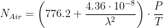 |
where
- P is air pressure [kPa].
- T is the air temperature [K].
 is the wavelength of light [cm].
Using the ideal gas law, we can show that temperature and pressure are closely related to density as shown in Equation 4.
| Eq. 4 |
 |
where
Equation 4 states that the ratio of P/T is proportional to  (R and MWAir are constants). This means we can restate Equation 3 in the simpler form shown in Equation 5.
| Eq. 5 |
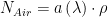 |
where
 is a function of the wavelength of light.
The index of refraction is a function of wavelength, as is shown in Figure 2. Note how the shorter wavelengths have a larger index of refraction than the longer wavelengths.

Figure 2: Air's Index of Refraction Versus Wavelength.
For this post, I will assume that the wavelength of light is fixed and that is a constant.
Air's Index of Refraction Rate of Change
For light to refract in the atmosphere, it must encounter air with an index of refraction that varies. The air's index of refraction is a function of its density, which varies with altitude and temperature. We can express the variation of the atmosphere's index of refraction using Equation 6.
| Eq. 6 |
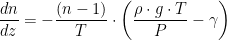 |
where
- n is the air index of refraction.
- z is the altitude.
- g is the acceleration due to gravity.
 is the atmospheric lapse rate, which is defined as the rate of temperature decrease with height (i.e.
  ).
).
Deriving this expression requires manipulation of the ideal gas law. The derivation is straightforward but tedious. I have included it in Appendix A.
Equation 6 has a couple of interesting aspects:
We can compute the autoconvective lapse rate as shown in Figure 3. The value I obtain here can be confirmed at this web page.

Figure 3: Calculation of the Autoconvective Lapse Rate.
Radius of Curvature for the Refracted Light Beam
Assuming a typical atmosphere, we can model the path of a refracted beam of light in the atmosphere as an arc on a circle. Figure 4 shows a derivation for the radius of curvature for a refracted beam of light. The radius of curvature will be constant (i.e. a circle) when  is a constant.

Figure 4: Derivation of the Radius of Curvature Expression.
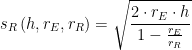
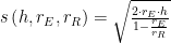
In the case of a lighthouse beam,  . This means we can write the refraction radius as
  .
.
Arc Length Traversed By A Refracted Light Beam
We are going to model the refracted light beam as moving along the arc of a circle of radius larger than that of the Earth. Figure 5 illustrates this situation.

Figure 5: Illustration of the Refracted Light Beam Moving Along the Arc of a Circle.
Given the geometry shown in Figure 4, we can derive an expression for the arc length upon the Earth's surface that the light beam traverses as shown in Figure 6.
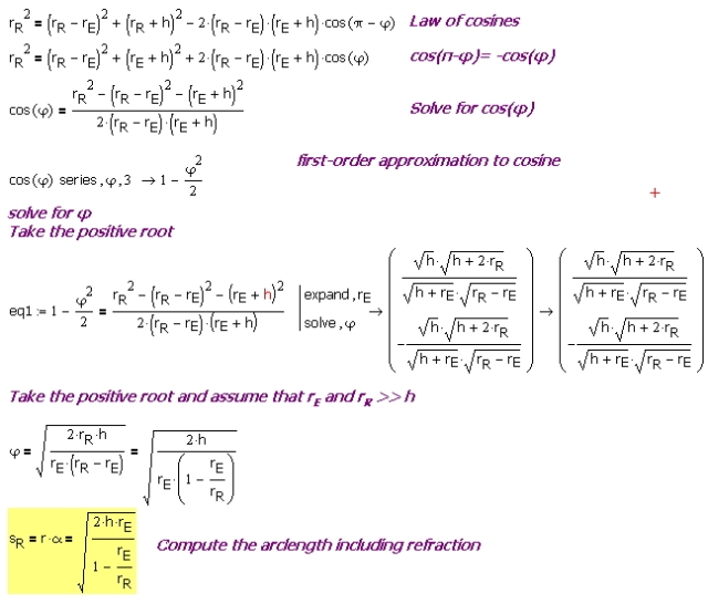
Figure 6: Derivation of Formula for the Distance Traveled Along the Earth's Surface By Refracted Light Beam.
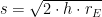
Equation 7 shows the key result from the derivation in Figure 6.
| Eq. 7 |
 |
where
- rE is the radius of the Earth.
- rR is the radius of the refraction circle.
- h is the height of the lighthouse.
Notice how Eq.7 can be viewed as Eq. 1 with an enlarged Earth radius of  . I see refraction often modeled by engineers who simply use Eq. 1 with an enlarged Earth radius. The radius used depends on the wavelength of the photons under consideration.
Simplified Arc Length Expression
Figure 7 shows how I obtained Equation 2 from Equation 7.

Figure 7: Equation 2 from Equation 7.
Conclusion
While the derivation was a bit long, I was able to derive Equation 2 from first principles. The derivation shows that the final result is sensitive to the choice of lapse rate, which varies throughout the day. I should note that the use of a refraction radius that is a multiple of the Earth's radius is often applied to other types of electromagnetic signals. For example, radar systems frequently use a "4/3 Earth radius" for refraction problems (Source). The refraction radius for radar is different than for optical signals because the index of refraction in the radio band is different from that of optical signals.
Appendix A: Derivation of Rate of Change of Atmospheric Index of Refraction with Lapse Rate.

Figure A: Derivation of Rate of Change of Atmospheric Index of Refraction with Lapse Rate.
Appendix B: Excellent Discussion of Index of Refraction, Lapse Rate, and Mirages.
I really like the way this author discusses mirages (Source).

Figure B: Excellent Description on the Formation of Mirages.
Save
Save
Save
Save


![\displaystyle d[\text{light-years }\!\!]\!\!\text{ =}\frac{{{d}_{AU}}[\text{km }\!\!]\!\!\text{ }}{\frac{\pi \left[ \text{radians} \right]}{180{}^\circ }\cdot \frac{\theta [\text{milliarcseconds }\!\!]\!\!\text{ }\cdot \text{0}\text{.001}\left[ \frac{\text{arcseconds}}{\text{milliarcseconds}} \right]}{3600\left[ \frac{\text{arcseconds}}{\text{degree}} \right]}\cdot {{d}_{LightYear}}[\text{km }\!\!]\!\!\text{ }}](https://s0.wp.com/latex.php?latex=%5Cdisplaystyle+d%5B%5Ctext%7Blight-years+%7D%5C%21%5C%21%5D%5C%21%5C%21%5Ctext%7B+%3D%7D%5Cfrac%7B%7B%7Bd%7D_%7BAU%7D%7D%5B%5Ctext%7Bkm+%7D%5C%21%5C%21%5D%5C%21%5C%21%5Ctext%7B+%7D%7D%7B%5Cfrac%7B%5Cpi+%5Cleft%5B+%5Ctext%7Bradians%7D+%5Cright%5D%7D%7B180%7B%7D%5E%5Ccirc+%7D%5Ccdot+%5Cfrac%7B%5Ctheta+%5B%5Ctext%7Bmilliarcseconds+%7D%5C%21%5C%21%5D%5C%21%5C%21%5Ctext%7B+%7D%5Ccdot+%5Ctext%7B0%7D%5Ctext%7B.001%7D%5Cleft%5B+%5Cfrac%7B%5Ctext%7Barcseconds%7D%7D%7B%5Ctext%7Bmilliarcseconds%7D%7D+%5Cright%5D%7D%7B3600%5Cleft%5B+%5Cfrac%7B%5Ctext%7Barcseconds%7D%7D%7B%5Ctext%7Bdegree%7D%7D+%5Cright%5D%7D%5Ccdot+%7B%7Bd%7D_%7BLightYear%7D%7D%5B%5Ctext%7Bkm+%7D%5C%21%5C%21%5D%5C%21%5C%21%5Ctext%7B+%7D%7D&bg=ffffff&fg=000&s=0&c=20201002)


![\displaystyle s\left[ \text{km} \right]=3.57\cdot \sqrt{h\left[ m \right]}](https://s0.wp.com/latex.php?latex=%5Cdisplaystyle+s%5Cleft%5B+%5Ctext%7Bkm%7D+%5Cright%5D%3D3.57%5Ccdot+%5Csqrt%7Bh%5Cleft%5B+m+%5Cright%5D%7D&bg=ffffff&fg=000&s=0&c=20201002)
 , where
  is the radius of the Earth.
![\displaystyle s\left[ \text{km} \right]=3.86\cdot \sqrt{h\left[ m \right]}](https://s0.wp.com/latex.php?latex=%5Cdisplaystyle+s%5Cleft%5B+%5Ctext%7Bkm%7D+%5Cright%5D%3D3.86%5Ccdot+%5Csqrt%7Bh%5Cleft%5B+m+%5Cright%5D%7D&bg=ffffff&fg=000&s=0&c=20201002)
 , where
  is the
 when
when 


