
Introduction
A phone call from a cancer epidemiologist a few months ago got me thinking radio communication over long distance. This researcher was a sharp guy who immediately saw the dynamic range issues associated with cell tower communication -- the issues are even worse for space communication.
I have always had a keen interest in radio communication. Two-way radios, for example, have so many unique advantages as they can be used where mobile phone reception is not reliable and they can also be used to ensure consistent and secure lines of communication between construction site workers and even the military. I know that you can find 2 way radios for sale in NYC, NJ & PA and many other states too, so, if you are looking for a walkie talkie, be sure to do plenty of research first to find the right one for you.
I recalled that I had archived some interesting paper articles years ago in my paper files (of course, indexed by an Access database I also wrote years ago). In these files I found an interesting Scientific American article on the difficulties involved with radio communication between the stars -- the article was written by a SETI researcher. There is "mathematical gold" to be mined in this article. This post just reviews the mathematics in this article. Let's dig in ...
Background
The article addresses three interesting types of problems:
- Estimating the Number of Stars Near the Sun
This problem involves making an estimate of the star density in the vicinity the Sun by using the Gliese Catalogue of Nearby Stars. Given the star density, we can compute the number of stars we would expect to find in a sphere of 100 light-years radius about the Sun.
- Computing the Power Required to Send A Clear Signal to All Stars Near the Sun Simultaneously
Here we compute the power required to drive a signal powerful enough to be received by all stars within 100 light-years distance of the Sun using an antenna that radiates power equally in all directions (i.e. isotropic radiator).
- Computing the Power Advantage of Beamforming
Using a large antenna, we can generate a very directional beam. This allows us to reduce our instantaneous power needs enormously, but we can only broadcast to a very narrow region of the sky. I have gone into beamforming basics in this post.
Analysis
Number of "Local" Stars
The analysis is pretty straightforward:
- Get a catalog of nearby stars.
There are numerous catalogs available -- just pick one that focuses on local stars.
- Find out how many stars are near the Sun.
I will use a 5 parsec (pc) neighborhood of the Sun to estimate the star density.
- Estimate the density of stars in the Sun's neighborhood.
I will assume this density is the same out to 100 light-years from the Sun. The idea here is that (1) we are more likely to have a good accounting of stars near the Sun that those further out because many stars are dim, and (2) the galaxy is so large relative to 100 light-years that the density of stars probably changes little out to 100 light-years.
- Estimate the number of stars in a 100 light-year neighborhood of the Sun.
Simply multiply the volume in a 100 light-year sphere by our estimate for the density of stars.
Figure 1 shows my Mathcad worksheet that estimates the number of stars within 100 light-years of the Sun. This analysis follows the approach of this source.

Figure 1: Estimate for the Number of Stars Within 100 Light-Years of the Sun.
Thus, there are likely over 14,000 stars within 100 light-years of our Sun.
Power for Driving an Isotropic Radiator over 100 Light-Years.
The article author computed the power needed to drive a readable signal based on the following assumptions:
- Assume the antenna is an isotropic radiator.
This assumption means that the radio power is projected equally in all directions -- the radio power distribution is spherically symmetric.
- Assume the receive antenna has aperture of 1 m2.
We have to make some assumption for the size of the receive antenna in order to estimate the amount of transmit power that will be received.
- The power is readable at 100 light-years distance.
Given a 1 m2 antenna aperture, this means that the signal level at 100 light-years is at the thermal noise level.
Figure 2 contains the calculation, which also shows that this transmit power is more than 5000 times greater than the total electrical power generation capacity of the United States.

Figure 2: Calculate the Power Needed to Communicate with a Star 100 Light-Years Away.
Beamforming's Power Advantage
Figure 3 shows the calculations associated with estimating the power advantage gained by using a large antenna with a very narrow, circular beam. This beam would be tough to steer accurately, but it would make the amount of power required substantially less. Unfortunately, you probably would only be able to send a signal to one star at a time.

Figure 3: Power Advantage Provided By Beamforming.
Conclusion
I have reviewed the calculations in the article and I was able to duplicate the author's results. This analysis shows the difficulty associated with radio communication between stars -- it is more than slow -- it takes power and/or an extensive antenna system.


![\displaystyle s\left[ \text{km} \right]=3.57\cdot \sqrt{h\left[ m \right]}](https://s0.wp.com/latex.php?latex=%5Cdisplaystyle+s%5Cleft%5B+%5Ctext%7Bkm%7D+%5Cright%5D%3D3.57%5Ccdot+%5Csqrt%7Bh%5Cleft%5B+m+%5Cright%5D%7D&bg=ffffff&fg=000&s=0&c=20201002)
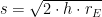 , where
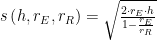
  is the radius of the Earth.
![\displaystyle s\left[ \text{km} \right]=3.86\cdot \sqrt{h\left[ m \right]}](https://s0.wp.com/latex.php?latex=%5Cdisplaystyle+s%5Cleft%5B+%5Ctext%7Bkm%7D+%5Cright%5D%3D3.86%5Ccdot+%5Csqrt%7Bh%5Cleft%5B+m+%5Cright%5D%7D&bg=ffffff&fg=000&s=0&c=20201002)
 , where n is the index of refraction. One common formula for the refractivity of dry air is given by Equation 3 (
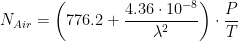
 is the wavelength of light [cm].
 , where
  is the
  is the air's density.
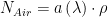
 is a function of the wavelength of light.
 is the atmospheric lapse rate, which is defined as the rate of temperature decrease with height (i.e.
  ).
). when
when 


 is a constant.
 . This means we can write the refraction radius as
  .
.


 is the temperature gradient [K/m] with respect to depth (d)
![\displaystyle {{q}_{Continent}}\approx 3.0\left[ \frac{\text{W}}{\text{m}\cdot \text{K}} \right]\cdot 20\left[ \frac{20\text{K}}{1000\text{ m}} \right]=60\frac{\text{mW}}{{{\text{m}}^{2}}}](https://s0.wp.com/latex.php?latex=%5Cdisplaystyle+%7B%7Bq%7D_%7BContinent%7D%7D%5Capprox+3.0%5Cleft%5B+%5Cfrac%7B%5Ctext%7BW%7D%7D%7B%5Ctext%7Bm%7D%5Ccdot+%5Ctext%7BK%7D%7D+%5Cright%5D%5Ccdot+20%5Cleft%5B+%5Cfrac%7B20%5Ctext%7BK%7D%7D%7B1000%5Ctext%7B+m%7D%7D+%5Cright%5D%3D60%5Cfrac%7B%5Ctext%7BmW%7D%7D%7B%7B%7B%5Ctext%7Bm%7D%7D%5E%7B2%7D%7D%7D&bg=ffffff&fg=000&s=2&c=20201002)


