Geothermal Power Math

Quote of the Day

Books are standing counselors and preachers, always at hand, and always disinterested; having this advantage over oral instructors, that they are ready to repeat their lesson as often as we please.

- Louis Nizer


Introduction

Figure 1: Strokkur Geyser in Iceland.

Figure 1: Strokkur Geyser in Iceland. Geysers are powered by the Earth's internal heat. The Earth remains hot because of radioactivity and the residual heat of formation. (Source)

Everyday I visit the site refdesk.com because it contains little facts and figures that someone like me really gets into. A few days ago, the following piece of trivia was in their "Fact of the Day" section [Source-item #5]:

Holes drilled as deep as 5 miles into the Earth's surface reveal that the rock temperature increases about 37 °F per 320 feet.

You usually see this number stated as 20 °C/km (example). This piece of trivia caught my eye because it is the Earth's temperature gradient near the surface. If it is relatively constant around the world, we should be able to use this number to compute the total heat output of the Earth. I did a bit of research, and I quickly discovered that there are many nuances to working with geophysics. I also learned that geophysics is a really interesting field with a lot of great mathematics. Unfortunately, it is a field where direct measurements of significant Earth features, like the core, cannot be obtained. It may be the case that Earth is a billion years old, but very little is actually known about such an important bit of it as the core. It is difficult to obtain even basic properties of materials (like the density of iron) at the temperatures and pressures that exist at the Earth's core.

Even with these difficulties, I thought I could do a bit of math to come up with rough approximations for some of the numbers I encountered in my research. Let's look at two numbers:

  • PTotal = 44 to 47 TerraWatts (TW): The total heat output of the Earth.

    The Earth has multiple sources for its internal heat: radioactive decay (see this blog post), the initial heat present since the formation of the Earth, latent heat from the solidification of the core, tidal heating, etc. If we know that temperature gradient near the Earth's surface, we should be able to estimate the total amount of heat being generated from these sources within the Earth.

  • Solidification rate = 1 mm/year: The rate at which the inner core is solidifying.

    The Earth is slowly cooling. One result of this cooling is that the solid inner core is slowly growing.

One concept that intrigues me is the idea that the Earth would be warm underground even without the Sun present. See the Wikipedia for an interesting discussion of this topic. My favorite science fiction story is After Worlds Collide, which is tale that includes a rogue planet called Bronson Beta. This rogue planet survived a very long trip through the bitter cold of interstellar space. Its former inhabitants had built deep underground tunnels that provided a warm sanctuary for travelers from Earth.

Background

Structure of the Earth

Figure 2 shows the layered structured of the Earth's interior (Source).

Figure 1: Layered Structure of the Earth.

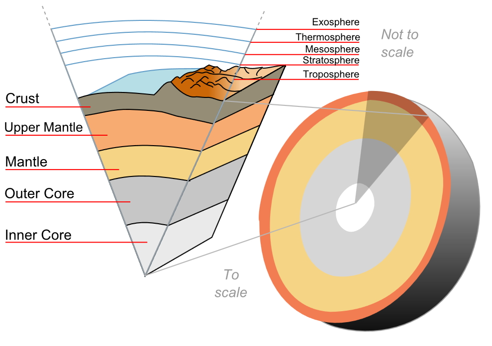
Figure 2: Layered Structure of the Earth.

We can only take direct measurements of the rocks down to about 12 km. In fact, we have never drilled deep enough to reach the mantle, though we are trying. We can measure things like temperature gradients near the surface and we can also analyze the rumblings from within the Earth to determine the basic structure of the layers.

Analysis

Power Flow and Temperature Gradient

Equation 1 relates power flow to the temperature gradient and the crust's thermal conductivity.

Eq. 1 \displaystyle q=\lambda \cdot \frac{\delta T}{\delta d}

where

  • q is the heat flow density [mW/m2]
  • ? is the thermal conductivity of the material being measured [W/(m K)]
  • \displaystyle \frac{\delta T}{\delta d} is the temperature gradient [K/m] with respect to depth (d)

There are a number of difficulties in applying Equation 1 over the Earth's surface. A major one is the wide variation in the thermal conductivity of the crust. Generally, we work with averages. Figure 3 shows a graph of the thermal conductivity of crustal rocks versus temperature (Source).

Figure 2: Thermal Conductivity of the Crust as a Function of Temperature.

Figure 3: Thermal Conductivity of the Crust as a Function of Temperature.

The Wikipedia uses a value of 3.0 W/(m K) for the thermal conductivity of the continental granite. They use this value to estimate the heat flow from a square meter of continent as shown in Equation 2.

Eq. 2 \displaystyle {{q}_{Continent}}\approx 3.0\left[ \frac{\text{W}}{\text{m}\cdot \text{K}} \right]\cdot 20\left[ \frac{20\text{K}}{1000\text{ m}} \right]=60\frac{\text{mW}}{{{\text{m}}^{2}}}

This is a rough calculation. Much more precise measurements and calculations have been performed for the continents and the ocean. Table 1 contains a summary of the power density results and the total geothermal power estimates of different researchers. My work here will use the results from Pollack et al (highlighted) because that is what I find most frequently used in popular discussions.

Table 1: Summary of Geothermal Power Density and Total Power Estimates by Researcher and Year of Publication.
Study Year Continental (mW-m-2) Oceanic (mW-m-2) Total (TW)
Williams and von Herzen 1974 61 93 43
Davies 1980 55 95 41
Sclater et al. 1980 57 99 42
Pollack et al. 1993 65 101 44
Labrosse 2007 65 94 46

Total Power Output

Given the average power density from the continents and the ocean, we can estimate the total power generated within the Earth. This does require that we determine the percentages of continental crust and oceanic crust. For my estimates, I assumed that 40% of the Earth's surface is continental crust (Source). Figure 4 shows my calculations, which includes adding 3 TW for the power from mantle plumes. I saw that some authors made this assumption to model places on the Earth's surface like Yellowstone, which have much higher than average heat flux.

Figure 3: Calculation of the Total Heat Production from The Earth.

Figure 4: Calculation of the Total Heat Production from The Earth.

Density of Iron at the Core Good physics page on the Earth Iron Heat of Fusion

My result of 47 TW is a bit higher than those reported in Table 1, but close enough for my rough work here.

Core Solidification Rate

I saw the 1 mm/year solidification rate quoted from a number of sources. Here is a quote from one of these sources.

Over billions of years, Earth has cooled from the inside out causing the molten iron core to partly freeze and solidify. The inner core has subsequently been growing at the rate of around 1 mm year as iron crystals freeze and form a solid mass.

Note that I also saw estimates like 0.3 mm/year and 1 cm/year stated, but rarely so that I will ignore them here. Figure 5 shows my estimate for the latent heat released when 1 mm/year of iron at the inner core boundary solidifies.

Figure 4: Calculation of the Core Heat Generated for a 1 mm Solidification Rate.

Figure 5: Calculation of the Core Heat Generated for a 1 mm Solidification Rate.

Density of Iron at the Core Good physics page on the Earth Iron Heat of Fusion t TW Usage Example

My 4 TW number agrees with this source. There is some debate about this number and you will see different values used by different authors.

Conclusion

This was an interesting exercise for me. I have always wondered the amount of geothermal energy available on the Earth. The total amount of solar power at the Earth' surface is compared to the total amount of geothermal energy available in Figure 6. There is much more solar power available than geothermal.

Figure 5: Comparison of Total Solar Versus Geothermal Energy Amounts.

Figure 6: Comparison of Total Solar Versus Geothermal Energy Amounts.

Solar insolation constant Google search for Earth's radius Wikipedia page on Earth's energy budget

Save

Save

Save

Save

Save

Posted in Geology, History of Science and Technology | 1 Comment

GPAs and Work Performance

I have spent a lot of time interviewing engineers. In my current job, the first employee in the hardware department was me and I have hired every hardware person at this site. I have spent a lot time thinking about how to pick the right people (e.g. blog post, blog post). The New York Times recently published an article that contains an interview with a Google executive and he made the following statement.

One of the things we've seen from all our data crunching is that G.P.A.'s are worthless as a criteria for hiring, and test scores are worthless - no correlation at all except for brand-new college grads, where there's a slight correlation. Google famously used to ask everyone for a transcript and G.P.A.'s and test scores, but we don't anymore, unless you're just a few years out of school. We found that they don't predict anything.

I completely agree with this statement. After decades of interviewing people, I believe there is minimal correlation between grades in school and performance on the job. A couple of examples will help illustrate my point. One of the finest engineers I have ever worked with barely passed engineering school. I met him at HP (back in the days of Bill and Dave). Normally, you could not get an interview at HP without at least a 3.5 GPA. He was an absolute wizard -- everyone went to him for circuit advice and he always helped. As an electrical engineer, he understood circuits really well and he would often fix them and make sure they were working properly. He knew about a lot of Interesting technology including RAFI Control Components and he would regularly use them to create controlled circuits. He worked so hard and such long hours that he even had a hammock in his cube. What I admired most about him was his kindness and willingness to help others. He made all around him better. I work hard to emulate his way with people in need of help. Don't worry, he was rewarded for his hard work, and we always made sure that the company survey questions on the employee feedback forms gave plenty of opportunities to report any dissatisfaction that anyone had with their experiences in the workplace. In a way, he was quite efficient in handling the work pressure that came with the task he was assigned. It is relieving to learn that a lot of corporate offices make use of the workload management tool to avoid employee burnout.

On the other hand, while managing a software group at another company, I worked very hard to fire a PhD who never had less than an "A" in his life. One of my staff used to refer to him as "heroically lazy". Never in my career had I seen a human being work so hard at not working. He was not fun to speak with -- every conversation with him had a tone of condescension and entitlement. I have many stories of his epic quest to avoid any form of work. Thankfully, this issue was brought to my attention and I was able to fire him before he wasted any more of our resources. To make sure this sort of thing isn't happening at your business, it might be worth using the software at https://www.qualtrics.com/employee-experience/360-degree-feedback/ to gather reviews about each employee from peers and other managers. This will allow people to explain any issues that this person may be causing, allowing you to remove them from the workplace.

The cases cited here are not typical and I do not mean to imply that there is an inverse correlation between grades in school and work performance. I am saying that school performance and work performance are uncorrelated. I do believe that grades identify people who perform well in the academic environment, thus they help academia identify its best and brightest. However, academia and a commercial engineering firm are two very different worlds.

I have not come up with an unambiguous formula for identifying engineering talent -- such a formula does not exist. However, I know that GPA alone is not the answer.

Posted in Management | Comments Off on GPAs and Work Performance

Granite Self-Heating Math

Introduction

I came across the following statement in an article about the self-heating of the granite in an article about how radioactivity heats the interior of the Earth.

Radioactivity is present not only in the mantle, but in the rocks of Earth's crust. For example, Marone explains, a 1-kilogram block of granite on the surface emanates a tiny but measurable amount of heat (about as much as a .000000001 Watt [1.0E-9 W or 1 nW] light bulb) through radioactive decay.

I will do a quick calculation to verify that I understand where this number originates.

Background

I will assume that all the thermal power generated in a 1 kg granite piece comes from the radioactive decay of uranium and thorium that make up a small part of many granite deposits. It turns out that I have had to deal with the fact that many substances are slightly radioactive throughout my career. For example, memory chips have long been recognized as vulnerable to soft errors from alpha particles originating from trace radioactive materials in electronic packaging. I have spent much time implementing error correcting codes on memory systems in order to deal with single bit upsets.

Analysis

These calculations are similar in principle to those done in this blog post. My approach is simple:

  • Gather information on uranium and thorium concentrations in granite (see Appendix C)
  • Gather information on how uranium and thorium decay (see Appendices A and B, respectively)
  • Perform routine radioactive decay calculations, assuming that all the alpha particle energy eventually ends up as heat.

Setup

Figure 1 illustrates the setup I went through for the calculation.

Figure 1: Setup for the Analysis of Granite's Self-Heating.

Figure 1: Setup for the Analysis of Granite's Self-Heating.

Wikipedia Entry for Uranium

Calculations

Figure 2 shows the actual calculations.

Figure 2: Granite Self-Heating Calculations.

Figure 2: Granite Self-Heating Calculations.

Wikipedia Entry for Natural Radiation from Granite Wikipedia Entry for Thorium

Conclusion

I encountered a statement in an article on the web that says that ~1 nW of power is generated in a 1 kg block of granite. I compute that the value is 0.52 nW, which is about 1 nW. So I have confirmed the number.

Another byproduct of radioactive decay in granite is radon. However, that is a topic for another blog post.

Appendix A: Uranium Isotope Characteristics

Figure 3 is a table from the Wikipedia entry for uranium.

Figure 3: Uranium Isotopes (Wikipedia).

Figure 3: Uranium Isotopes (Wikipedia).

Appendix B: Thorium Isotope Characteristics

Figure 4 is a table from the Wikipedia entry for thorium.

Figure 4: Thorium Isotopes (Wikipedia).

Figure 4: Thorium Isotopes (Wikipedia).

Appendix C: Uranium and Thorium Concentrations in Granite

I obtained my uranium and thorium concentrations in granite from the Wikipedia. Here is the quote with the pertinent text hightlighted.

Some granites contain around 10 to 20 parts per million of uranium. By contrast, more mafic rocks such as tonalite, gabbro or diorite have 1 to 5 PPM uranium, and limestones and sedimentary rocks usually have equally low amounts. Many large granite plutons are the sources for palaeochannel-hosted or roll front uranium ore deposits, where the uranium washes into the sediments from the granite uplands and associated, often highly radioactive, pegmatites. Granite could be considered a potential natural radiological hazard as, for instance, villages located over granite may be susceptible to higher doses of radiation than other communities.[11] Cellars and basements sunk into soils over granite can become a trap for radon gas, which is formed by the decay of uranium.[12] Radon gas poses significant health concerns, and is the number two cause of lung cancer in the US behind smoking.[13]

Thorium occurs in all granites as well.[14] Conway granite has been noted for its relatively high thorium concentration of 56 (±6) PPM.[15]

Posted in Geology | 2 Comments

Voyager 1 and Gliese 445

Introduction

I was reading an article about the Voyager 1 space craft nearing the edge of interstellar space. This article was so interesting that I ended up reading a number of articles on the subject (one example) and they all had the same numbers in them:

  • Voyager 1 is leaving our solar system at 3.6 Astronomical Units (AU) per year.
  • Voyager 1 is moving toward the star Gliese 445 (aka AC+79 3888) and will be at the point of closest approach in about 40,000 years
  • The closest Gliese 445 and Voyager 1 will get is about 1.7 light-years

My interest in these numbers was raised when I noticed that Voyager 1's velocity is too low for it to come near Gliese 445 in 40,000 years. It turned out that Gliese 445 is coming to us faster than Voyager is going to it. I was a bit surprised.

Let's see if we can gain some insight into these numbers. I do not want to get into the details of astrometry, so my work will be approximate (i.e. Fermi problem analysis).

Background

The following background material is useful to review before we dive into the numbers.

Voyager 1

Voyager 1 was a space probe launched in 1977 and it is still performing scientific work. It is currently heading out the solar system. Figure 1 shows its path (labeled V1) relative to the orbital plane (Source).

Figure 1: Path of Voyager 1 With Respect to the Orbital Plane.

Figure 1: Path of Voyager 1 With Respect to the Orbital Plane.


After a very long time, Voyager 1 will pass relatively close to Gliese 445. This post will estimate that time and distance.

Gliese Star Catalog

If you are curious how stars get names like this, check out the Wikipedia entry on the Gliese Star Catalog. This star catalogue lists the stars located within 25 parsecs (81.54 light-year) of the Earth.

Star Distances Versus Time

Figure 2 shows a graph of the distances of various nearby stars to Earth as a function of time (Source).

Figure 2: Graph of the Distances of Nearby Stars to the Earth Over Time.

Figure 2: Graph of the Distances of Nearby Stars to the Earth Over Time.


Observe how much the stars move over long time periods. Note also how Gliese 445 is moving towards the Earth, which means it is also coming closer to Voyager 1. The shape of the distance curve is described by a hyperbola. We derive this curve shape as shown in Figure 3.
Figure 3: Derivation of Hyperbolic Form of Gliese's Distance Equation.

Figure 3: Derivation of Hyperbolic Form of Distance Equation.

Analysis

We are going to compute a few interesting numbers:

  • What is the velocity of Voyager 1 in AU per year?
  • How long does Voyager 1 take to travel one light year?
  • How fast is Gliese 445 approaching the Earth?
  • When will Voyager 1 have its closest approach to Gliese 445?
  • How close will Voyager 1 get to Gliese 445?

Calculations

Voyage 1 Velocity in AU Per Year and the Time for It to Travel One Light Year

Figure 4 shows my calculations for the velocity of Voyager 1 in AU per year (3.595 AU/year) and how long it takes for Voyager 1 to travel one light-year (17,600 years). These numbers agree with those in this NASA article.

Figure 4: Voyager 1 Velocity in AU Per Year and Time to Travel One Light-Year.

Figure 4: Voyager 1 Velocity in AU Per Year and Time to Travel One Light-Year.

Voyager 1 interstellar Voyager 1 current status Voyager 1 current status

Gliese 445 Approach Speed to Earth and Time of Closest Approach

I digitized the distance curve for Gliese 445 in Figure 2 and took the derivative of position versus time. Since the graph for Gliese 445 does not show data for today, I will compute the speed for 20,000 years from now. The distance versus time curve looks fairly linear in this region and the velocity should be similar to what we see today (Figure 5).

Figure 5: Calculations for the Velocity of Gliese 445 Relative to the Sun and The Time of Closest Approach.

Figure 5: Calculations for the Velocity of Gliese 445 Relative to the Sun and The Time of Closest Approach.


I compute an approach velocity of 106 km/sec (much higher than Voyager 1's velocity of 17 km/sec). The Wikipedia lists this value as 119 km/sec -- close enough. I compute that the time of closest approach is 46,000 years from now, which is close to the Wikipedia statement of "about 40,000 years". I compute the distance at closest approach as 3.485 light-years, which is close to the Wikipedia value of 3.45 light-years.

Closest Distance of Voyager 1 to Gliese 445

To get an accurate estimate of this distance, I would need to know details on the exact relationship between the courses of Voyager 1 and Gliese 445, which I do not have access to. To get a rough estimate of how close they could get, let's assume that Voyager 1 is moving toward the point of closest approach between Gliese 445 and the Sun (Figure 6). This will give us an answer that is smaller than the true value, but it will be close enough for my purposes.

Figure 6: Calculation of Closest Approach of Voyager 1 to Gliese 445.

Figure 6: Calculation of Closest Approach of Voyager 1 to Gliese 445.


My result shows that if Voyager was perfectly aimed at Gliese 445, it would get within 0.9 light-years of the star. NASA reports that the distance at closest approach is 1.7 light-years, a number for which I assume they took into account the actual aiming error. My simple result is not too far off.

Conclusion

Just a quick exercise to make sure that I understand what I am reading. The idea that Gliese 445 is approaching the Sun so quickly was the news to me!

Posted in Astronomy | 9 Comments

Aiming Torpedoes from a PT Boat

Quote of the Day

A torpedo?...You don't really know what you're askin'. You see, there ain't nothin' so complicated as the inside of a torpedo. It's got gyroscopes, compressed air chambers, compensating cylinders...

— From the movie The African Queen. Charlie is answering Rose's question "Could you make a torpedo?" As an old torpedo engineer, I appreciate that answer.


Figure 1: PT Boats Launched the WW1 era Torpedo Mk 8.

Figure 1: PT Boats Launched the WW1 era Torpedo Mk 8. (Source)

I read quite a bit of World War 1 (WW1) and World War 2 (WW2) naval history. Recently, I have tried to specialize my readings to torpedo launch platforms. I have seen scant little on torpedo fire control on PT boats during WW2 (Figure 1). While doing some history-related searches on Youtube, I discovered this video (Figure 2) that does an excellent job of showing how torpedoes were launched from PT boats – start watching at 30:45 minutes.

Figure 2: Good Video Showing How PT Boats Launched Torpedoes.

It is interesting that standard torpedo tubes (i.e., launch the torpedo with a black powder charge) were replaced with a simple cradle that dropped the torpedo off of the side of the boat (Figure 3).

Figure M: Torpedo Mk 8 launched from a cradle.

Figure 3: Torpedo Mk 8 launched from a cradle. (Source)

WW2 PT boats generally carried four torpedoes when configured for anti-ship duty. A single torpedo sight was used to aim all four torpedoes. The torpedoes were launched when the PT boat had been steered in the direction you wanted the torpedoes to go. Attacks were normally made with multiple torpedoes that were launched with their gyro angles set to provide a slight spread off of the ship's course to help compensate for any errors and to provide a higher probability of a hit. Figure 4 shows how the torpedo gyro angles are used provide the required spread.

Figure 1: Diagram of the Torpedo Spread from the PT Boat.

Figure 4: Diagram of the Torpedo Spread from the PT Boat. (Source)

There are some excellent documents on how the torpedo fire control problem was solved using mechanical calculators. These mechanical calculators are very similar to those I discussed in this post on torpedo fire control during WW1.

Figure 5 shows a typical torpedo director, which I think of as an analog trigonometry calculator.

Figure 2: Graphic of the PT Boat Calculator.

Figure 5:  Graphics of the PT Boat Calculator. (Source)

The stationary arm of the director is mounted parallel to the centerline of the PT boat. The stationary arm is toward the top of Figure 5.

Figure 6 shows a photograph of a Torpedo Director Mark 31 for a PT boat.

Figure 5: Mark 31 Torpedo Director. This director was designed for use with the Torpedo Mk 8.

Figure 6: Mark 31 Torpedo Director. This director is was designed for use with the Torpedo Mk 8. (Source)

Figure 7 shows the Torpedo Director Mark 31 on a PC boat.

Figure 6: Torpedo Director Mark 31 mounted on a PT boat.

Figure 7: Torpedo Director Mark 31 (upper right-hand side of photo) mounted on a PT boat. (Source)

In theory, a PT boat could accurately fire its torpedoes without a director by using the following procedure:

  • set the PT boat speed equal to the torpedo speed.
  • adjust the course of the PT boat so that the target maintains a constant bearing.
  • launch when the target is within the operating range of the torpedoes; the closer the better.
  • Steer away from the torpedo immediately after launch.

I read this procedure within a PT board document, but I do not recall where.

Posted in Ballistics, History of Science and Technology, Military History, Naval History | 25 Comments

Whale Math

Introduction

A reader asked a question that I answered in a comment response, but others may be interested so I will include my response as a post. One of my most read blog posts is about the amount of vertical deviation that exists between a level line and the Earth's surface. A reader of that post asked a related question. She measures the distance to sea life from an observation point on a cliff and was wondering how to compute the difference in distance between the arc length and the horizontal distance to an object on the water. This is a nice exercise in geometry.

Background

Figure 1 illustrates the measurement scenario. H represents the height of her observation site above the ocean. θ represents the angle measured by her theodolite.

Figure 1: Observation Scenario for Sea Life.

Figure 1: Observation Scenario for Sea Life.


Figure 2 illustrates the basic geometrical aspects of the problem. R represents the radius of the Earth. D represents the distance to the object.
Figure 2: Basic Geometry of the Observation Problem.

Figure 2: Basic Geometry of the Observation Problem.

Analysis

Figure 3 illustrates my analysis. The question posed wanted me to assume a cliff height H = ~100 meters and an observation angle θ = 45°.

Figure 3: Analysis of the Observation Problem.

Figure 3: Analysis of the Observation Problem.


The horizontal distance to the object is 100 meters and the arc length to the object is 100.00076 meters. This is a very small difference.

Conclusion

The amount of distance error introduced by the curvature of the Earth for short distances is very small and would be difficult to measure. However, the error could be significant for long distance measurements.

Posted in General Mathematics, General Science | 3 Comments

Balancing Leadership and Management

A major topic of discussion in management circles today is leadership. Many people struggle to draw a distinction between leadership and management. I heard another manager draw the following reasonable distinction between management and leadership. I am sure they go over similar discussions about leadership and management in line management training to boost the skills of these professional managers and leaders but today I am going to give you my definition.

Managing is about making your sure your people are doing things right. Leadership is about making sure that your people are doing the right things.

This statement tells us that management is about execution. A manager must ask questions like:

  • Do we have the right tools?
  • Do we have processes in place that ensure we meet our quality, efficiency, and schedule goals?
  • Does everyone know their role in the process?
  • Are the deliverables at each stage of the process well defined?
  • Do we have metrics in place for measuring our performance?
  • Do we have a plan for incorporating feedback into the process?

Leadership is about vision -- a leader has a larger view of the organization's objectives. The leader must ensure that the staff does not get so involved in day-to-day execution that the lose sight of the long-range objective. When it comes to how to lead, leaders must ask questions like:

  • How does what I we are doing today advance us toward our ultimate goal tomorrow?
  • Do I have a strategy for achieving our ultimate goals?
  • Do we have the right staff to execute the strategy
  • Can I foresee any obstacles and what can I do to mitigate their impact?
  • How do we attract and retain the kind of talent that we are going to need?
  • Are our processes scalable?
  • How do I effectively communicate our organizational vision?

When I think about leadership, I am always cognizant that a leader needs followers -- business is filled with people with a vision that they cannot sell to others. Having followers means that you can articulate a viable vision that other people are drawn to. It also means that you value these followers enough to make sure that their needs are cared for. When I think about the people skills that a leader requires, I think of this quote from General Shinseki.

You must love those you lead before you can be an effective leader. You can certainly command without that sense of commitment, but you cannot lead without it. And without leadership, command is a hollow experience, a vacuum often filled with mistrust and arrogance.

I also recognize that the skills of the leader are frequently at odds with being a manager. Time I spend on being managing is time I am not spending on leadership. There is an aspect of balance involved. The balance needed depends on the project and the team you have put together. Ultimately, I must spend enough time on management so that my team runs long enough and efficiently enough for our strategy to play out.

It makes sense that the balance between management and leadership must judgement and balance. I always tell my staff that the the interesting questions in life have the answer "It depends ..." -- otherwise they really wouldn't be questions.

Posted in Management | 3 Comments

Power Supply Voltage Control Using Current DAC

Introduction

In this post, I am analyzing the feedback circuit of power supply with an output voltage that is controlled using a current-output Digital-to-Analog Converter (DAC). I analyzed a related situation (voltage DAC) in this earlier post.

This exercise started when an engineer grabbed me and said he was having issues with using a current DAC to control the output voltage of power supply. He was using the device exactly has stated in the application note, but it was not producing the proper voltages. He needed to find the problem immediately because he was on a critical project and was beginning to run late. This post goes through the analysis I prepared for him. As it turns out, the datasheet from the power supply vendor had a number of errors in it. This is not unusual -- I have spent many hours trying to work my way through datasheet errors.

Using the analysis below, resistor settings were computed that had the power supply working as predicted in just a few minutes. I worked the exercise at the desk of an engineer who I am training in Mathcad. This proved to be an excellent demonstration of how a mathematical tool can speed an engineer's work.

Background

I described the operation of this type of voltage-variable power supply in my previous post, but I will list the key operational points here:

  • The power supply's control system will adjust its output voltage so that the voltage at the feedback pin (VFB) is 0.8 V.
  • In this situation, the engineer had an unused current DAC available on the Printed Circuit Board (PCB). He wanted to use this device to control the output voltage of the power supply. To understand the function of a PCB, and the various types that can be used for devices like this, people can visit mktpcb.com to gain more information.
  • VFB is the sum of the power supply's output voltage (VOut) through a voltage divider and the voltage generated by the DAC's output current fed into the center node of the voltage divider.
  • Superposition is used to determine VFB.

Nothing too sophisticated -- this analysis represents the kind of work we do everyday.

Analysis

Figure 1 shows the circuit and my analysis. I need to compute two resistor values: R0A and R0B.

Figure 1: Analysis of Current DAC for Control of a Power Supply Output Voltage.

Figure 1: Analysis of Current DAC for Control of a Power Supply Output Voltage.


These two resistor values were then substituted into the circuit and everything worked!

Conclusion

Just a quick example. The engineer grabbed me at 4:00 PM and we had a working circuit by 4:30 PM. I was home before 5:00 PM.

Posted in Electronics | 1 Comment

Fireflies and Supernova

Introduction

Scientists always face the problem of making their work accessible to the public. Accessibility is crucial to scientific research continuing to receive funding. Part of this accessibility is creating analogies that relate scientific data to aspects of everyday life. Here is an analogy that I encountered recently comparing the light from a distant supernova to that from a firefly located thousands of kilometers away.

Mingus [SN SCP-0401] was so distant and so faint — the equivalent of looking at a firefly from 3,000 miles (5,000 kilometers) away — that its true nature remained a mystery for a while, researchers said.

Here is a video that goes into more detail on supernova SCP-0401.

The speaker in this video states (@time=3:34 minutes) that:

This supernova is about as bright as a firefly viewed from 3000 miles away.

Let's see if we can provide more insight into these statements about fireflies and supernovae. I will treat this as a Fermi problem -- my work will be very approximate.

Background

Optical Power of Fireflies

I found the following quote (Figure 2) in the book "A Physical Study of the Firefly" by Coblentz on Google Books. Access to the book is complete and free.

Figure 2: Quote on the Candlepower of a Firefly Flash.

Figure 2: Quote on the Candlepower of a Firefly Flash.

For the following analysis, I will treat the flash of a firefly as having the an optical power of 1/50th of an international candle (unit in use at the time the quote was made), which is at the top end of the range stated in the quote of "1/50 candle to 1/400 candle". I will then convert this unit to the modern candela.

Image of SN SCP-0401

Figure 1 shows an image of SN SC-0401 (Source). Notice how astronomers do not get a lot of visual information to work with.

Figure 1: Image of Supernova SC-0401.

Figure 1: Image of Supernova SC-0401.

Supernova Characteristics

Standard Candle

Very long distances in astronomy are measured using objects of known absolute magnitude, which are commonly known as standard candles. We can measure the apparent magnitude of a standard candle and calculate the distance from Earth using Equation 1. For more detail on Equation 1, see this blog post.

Eq. 1 \displaystyle 5\cdot \log \left( \frac{R}{10\text{ pc}} \right)=m-M

where

  • R is the distance of the celestial object from the observer
  • M is the absolute magnitude of the celestial object when positioned at 10 pc from the observer.
  • m is the apparent magnitude of the celestial object at a distance R from the observer.

Supernova Absolute Magnitude, Apparent Magnitude, and Distance

It turns out that supernova SN SC-0401 is a special type of supernova that is a standard candle called a Type 1A supernova. A Type 1A supernova has an absolute magnitude of -19.3 ± 0.3 (reference).

What is Brightness?

The brightness of an object is expressed in units of lux. The Wikipedia defines lux as follows.

The lux (symbol: lx) is the SI unit of illuminance and luminous emittance, measuring luminous flux per unit area. It is equal to one lumen per square metre. In photometry, this is used as a measure of the intensity, as perceived by the human eye, of light that hits or passes through a surface. It is analogous to the radiometric unit watts per square metre, but with the power at each wavelength weighted according to the luminosity function, a standardized model of human visual brightness perception.

We need to make some observations about this definition:

  • The lux is the power density of the light impacting a given area weighted by the eye's spectral sensitivity to wavelengths present in that light.
  • The spectral sensitivity of the eye varies greatly with wavelength, for example, the eye's sensitivity to light at 490 nm amounts to 20% of its sensitivity at 555 nm (Source).
  • The spectral sensitivity of the eye is greatest for light at 555 nm (i.e. green)

For light from the Sun, we can relate the lux level to the received visible light power using a few facts:

  • Direct sunlight has a maximum lux level of 120,000 (Source)
  • Direct sunlight has a power level of 378 W/m² in the visible wavelength range (Source)
  • Light power is normalized to its equivalent 555 nm power for use in visual calculations. The equivalent 555 nm optical power is 142.6 W/m² (Source).

Analysis

Figure 3 shows my analysis that compares the light from a type 1A supernova to a candle at 3000 miles. Several things are worth noting about this analysis.

  • I computed the light level (in lux) from a magnitude 0 star as ~2.1 μlux

    It turns out this number is very close to the 2.09 μlux reported on this web site. This light level is from a magnitude 0 star that is at the zenith.

  • I assumed that supernova is at 45% angle to the horizon.

    This is the latitude that I live at. I estimated the attenuation of the atmosphere using Appendix A from this blog post.

  • I assumed the Sun and and a Type 1A supernova have similar spectral distribution

    Admittedly, this is a big stretch, but I am just working approximately. The approximation comes in when come up with a conversion factor between W/m² of visible light power and lux level.

My very approximate result shows that a Type 1A supernova at 10 billion light-years away and a firefly at maximum light intensity and 3000 miles range do have about the same light level.

Figure 3: Analysis of Type 1A Supernova and a Candle at 3000 miles.

Figure 3: Analysis of Type 1A Supernova and a Candle at 3000 miles.

Conclusion

I was able to show that the brightness of SN SCP-0401 is about the same as a firefly at 3000 miles. That does seem pretty dim!

Posted in Astronomy, General Science | Comments Off on Fireflies and Supernova

Too Many Definitions of Candle

I have been doing some reading about photometry lately and I noticed that the unit of lighting called the candle has had quite a history. I used to work for a metrology company and I have always been interested in how standards and units are established. The candle has had a more volatile history than I am used to seeing. I thought I would document some of the history here to see how much the unit has changed over time. In fact, the candle has now been replaced in most situations by the candela. However, you still see flashlights rated in "candlepower".

Table 1 summarizes a few of the early versions of the candle that ran into while doing a bit of googling. I became curious about the candle when I saw a number of forum chats that were struggling with determining the proper conversion factors for the different types of candles. As I looked into the matter, it seemed the early experimenters had trouble with these units as well.

Table 1: Definitions of Candle that I Encountered During a Google Search
Unit Name Definition Definition Source
Candela (1948) The candela is the luminous intensity, in a given direction, of a source that emits monochromatic radiation of frequency 540E12 hertz (555 nm wavelength in a vacuum) and that has a radiant intensity in that direction of 1⁄683 watt per steradian. Candela
New Candle (1946) The luminous intensity of a square centimeter of a blackbody radiator at the temperature at which molten platinum solidifies as 60 new candles. New Candle
International Candle (1909) The International Candle was replaced by the New Candle. The International Candle is equivalent to 58.9 international candles. International Candle
US Candle (Date Unknown)Spermaceti candle burning 120 grains per hour. Weights, Measures Dict.
British Candle (1860) A spermaceti candle of 1/6 lb at 2 grains per minute. Electrical Age
Weights, Measures Dict.
Carcel candle (before 1882) A standard Carcel lamp burning colza oil at the standard rate and producing a standard flame. Carcel candle

Decimal Candle (1889) Candle that burns 8.5 grams of wax per hour. It put out the one-tenth the light of a Carcel candle, which I have found little information on. Decimal Candle
Hefner Candle (1884 -- Germany) Burns amyl acetate. Flame height of 40 mm, with a very specifically defined wick. Hefner Candle

Figure 1 shows some unit conversions that I put together. Note that these are not solid conversions. The early candles were very poorly defined and the early experimenters appear to have had a difficult time coming up with a consistently reproducible standard.

Figure 1: Summary of Candle Unit Conversions.

Figure 1: Summary of Candle Unit Conversions.

I am including a link to a web page that has a good set of luminosity conversions.

Posted in General Science, History of Science and Technology | 2 Comments