Quote of the Day
A nation is a society united by a delusion about its ancestry and a common hatred of its neighbors.
— William R. Inge. There are days when this seems very true …
Introduction
I have been reading a couple of excellent books about battleships ("Naval Firepower" and "Guns at Sea"). During my reading, I have encountered the term "Danger Space" that appears with nearly every table describing the large naval guns. Of course, I had no idea what danger space was when I began investigating it. It turns out that danger space describes an important metric for battleship guns, and it is worthwhile documenting what I have learned about it here.
There appears to be a number of ways to define danger space. Since my reading is on US battleships, I will focus on the how the US Navy used the term. All the world's navies had closely related definitions for danger space that ended up producing slightly different numerical results. My plan in this post is to:
- define danger space as used by the US Navy
Some definitions use the width of the ship (referred to as the beam -- see Appendix D for an example) and some don't. Some use different target height standards (e.g. 20 feet versus 30 feet). I believe that I now understand the need for the different forms -- it has to do with your priorities. For example, if your priority is to blow through the heavily armored regions from the side, the width of the ship is not very important. If you plan on dropping shells down on the deck, the width of the ship becomes important. For more discussion of this topic, see this discussion of the zone of immunity.
- derive the formula(s) used to compute it
I am not totally happy with my derivation, but it is what I could come up with. I am sure that the originators were working with approximations and they were trying to get answers that were reasonably close and easily computable by hand.
- provide evidence that the formula I am using is the same as used by the US Navy
US Navy range tables do not state the formula used to determine the danger space. I will compare the results using the formula that I found with the US Navy's published results.
I list the references I used at the bottom of the blog post. I should mention that there are numerous synonyms for danger space:
- danger zone
- hitting space or zone
- bestrichener raum ("smear space" – my translation)
Background
The Motivation for Danger Space
Obtaining hits with long-range naval gunnery is closely tied to minimizing errors in determining the target's range. Range errors are usually larger and more difficult to correct than deflection errors (details here). Danger space tells us the amount of range error we can tolerate and still hit our target. Given that there are always errors present in our target range measurements, having a gun with a large danger space means that you have a greater chance of hitting your target for a given number of shells fired.
Definition of Danger Space
Danger space is also tied in with the concept of a citadel. Most analysts only focus on hits to the vital areas of the ship. On battleships, the vital areas were heavily armored and were referred to as the citadel. The US Navy usually assumed a citadel height of 20 feet2 -- the British Navy used 30 feet3. The length of the citadel varied with the type of target. The key concept here is that target range errors less than the danger space will still produce hits on the citadel.
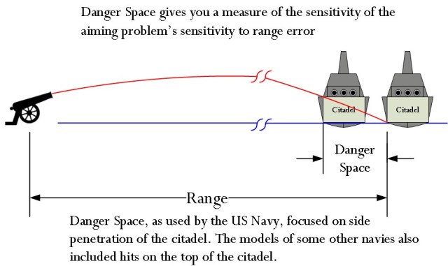
Figure 1: Danger Space Illustration.
Figure 1 illustrates how the danger space is about putting a projectile through the citadel our a range interval. Given this viewpoint, Algier1 gives the following definition for danger space. A similar definition is presented here.
By the term “danger space” is meant an interval of space, between the point of fall and the gun, such that the target will be hit if situated at any point in that space. In other words, it is the distance from the point of fall through which a target of the given height can be moved directly towards the gun and still have the projectile pass through the target. Therefore, within the range for which the maximum ordinate of the trajectory does not exceed the height of the target, the danger space is equal to the range, and such range is known as the “ danger range.”
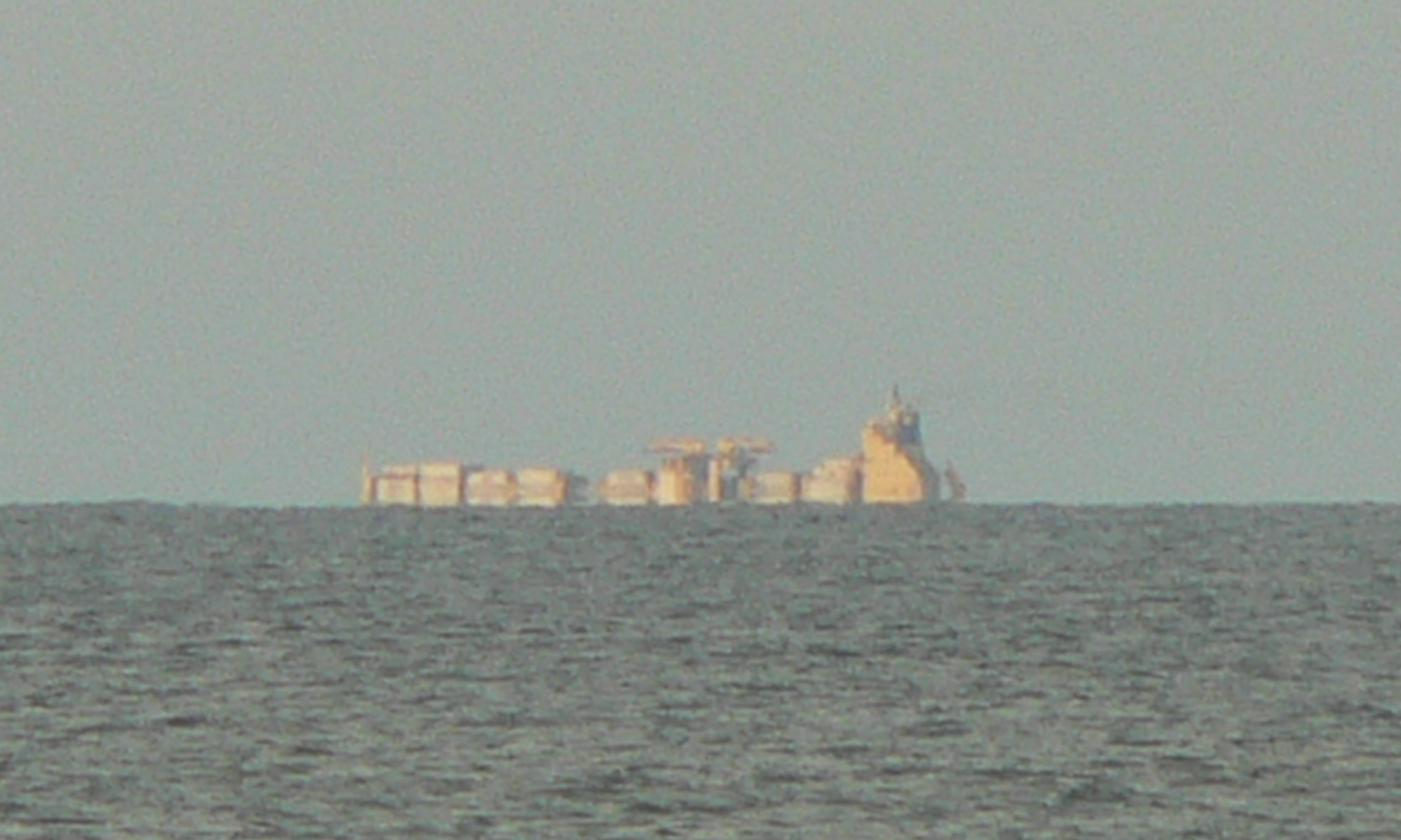
Note that the focus of this definition is on the projectile passing through the target (i.e. the vertical face of the citadel), not dropping onto the target (i.e. the top of the citadel). You see the effect of this viewpoint by examining how US Navy towed gunnery targets were constructed (Figure 2). There were a number of different size targets used (Figure 3). Because the US Navy was less interested in hits on the top of the citadel, the targets were very narrow in thickness.
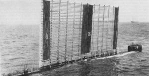 Figure 2: Example of a World War 2 Towed Gunnery Target. |
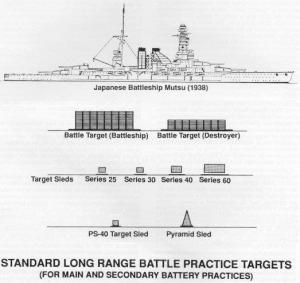 Figure 3: Sizes of US Navy Towed Gunnery Targets. |
There are some important observations that you need to make about this definition of danger space.
- Long range engagements are miss-prone because at long-range the projectiles have large fall angles, resulting in small danger spaces.
- Short range engagements tend to have more hits because projectiles have shallow fall angles, resulting in large danger spaces.
- At some short range, your danger space will equal your range because the projectile is traveling with such a shallow angle that a hit is guaranteed.
Analysis
Danger Space Equation
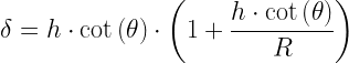
Algier1 gives Equation 1 for danger space. I make an attempt at a derivation for Equation 1 in Appendix A. Deriving Equation 1 requires making an approximation for the change in fall angle over the danger space interval.
| Eq. 1 |
 |
where
- δ is the danger space.
- θ is the fall angle (i.e. the projectile's angle of descent at the point of impact).
- R is the target range.
- h is the target height.
There are a couple of special points worth making about Equation 1:
- The only target characteristic present in Equation 1 is height.
The US Navy was only interested in side penetration of the citadel. I have seen the danger spaces for guns of other navies listed where the width of the ship appeared to be included the calculation. Note that I drew Figure 1 showing the projectile striking the citadel broadside. The tactics of the day would have preferred to cross the T (i.e. target bow is facing the attacker). Citadel height is still the important parameter in this case. However, the citadel length now would be important for strikes on the top of the citadel.
- In the case where
 , Equation 1 reduces to
  .
.
Some authors do mention as a useful approximation. This approximation is equivalent to assuming that the path of the shell over the danger space is a perfectly straight line. See Appendix C for a reference example from a Royal Navy document.
Equation 1 can be solved for danger space to give a quadratic. The solution for the quadratic is given by Equation 2.
| Eq. 2 |
 |
Because of the hand computation difficulties associated with Equation 2, we can approximate the term R/(R-δ) in Equation 1 using a one-term series expansion to obtain Equation 3 (derivation shown in Appendix B). However, the result is not particularly accurate at short ranges. Equation 3 is also given by Algier1.
| Eq. 3 |
 |
Comparison with World War 2 Publications
I have worked numerous examples from various books. I have included two here that are representative. They come from this document. For those who are interested, my spreadsheet is included here.
Comparison with 16 in/45 or 50 Caliber Range Table for 2700 lb Shell
I am mainly interested in Iowa and South Dakota classes of battleships, which used 16-in guns (50 caliber and 45 caliber respectively). I will use their range tables for examples.
Figure 4 shows a screenshot of an Excel worksheet using both Equation 2 (quadratic solution) and Equation 3 (approximate solution). Equation 2 gave me very nearly the same results as listed in the reference publication.

Figure 4: Duplication of Results From Abridged U.S. Navy Range Table (2700 lb Shell, 45/50 Caliber).
Comparison with 16 in/45 Caliber Range Table for 1900 lb Shell
Figure 5 shows a screenshot of an Excel worksheet using both Equation 1 (quadratic solution) and Equation 2 (approximate solution). Equation 1 gave me very nearly the same results as listed in the reference publication.

Figure 5: Duplication of Results From Abridged U.S. Navy Range Table (1900 lb Shell, 45 Caliber).
Conclusion
I believe that I have shown how the danger space was computed by the US Navy during World War 2. Danger space is most often seen today in the context of small arms.
References
1Philip Algier, The Groundwork of Practical Naval Gunnery, Annapolis, MD: The United States Naval Institute, 1917, pp 59-65.
2Abridged Range Tables for U. S. Naval Guns. Washington, D.C.: Navy Department Bureau of Ordnance, 1944, p59.
3Friedman, Norman. Naval Firepower: Battleship Guns and Gunnery in the Dreadnaught Era. Annapolis: Naval Institute Press, 2008.
Appendix A: Derivation of Equation 1
Figure 6 shows the basic geometry associated with my derivation of Equation 1. I have no idea if this is how Equation 1 was originally derived, but this is the approach I chose to use.

Figure 6: Graphic Illustrating the Danger Space Geometry.
Figure 7 shows the actual mathematical details of the derivation.

Figure 7: My Derivation of Equation 1.
Appendix B: Simplification of Equation 1 into Equation 3
Figure 8 shows how the approximations used to derive Equation 3 from Equation 1.

Figure 8: Derivation of Equation 2.
Appendix C: Royal Navy Excerpt on Danger Space
Early Royal Navy documents referred to "dangerous distance" instead of "danger space". Figure 9 shows an excerpt from the "Textbook of Gunnery" dated 1902.

Figure 9: Royal Navy Reference on Danger Space.
Appendix D: US Navy Excerpt That Uses the Beam of the Ship
Figure 10 shows a snippet from an old US Navy document. This one is unusual in that it includes the beam of the ship in the equation.

Figure 10: One Form of Danger Space That Uses Ship's Beam.


 less light is available at Mars than at the Earth.


