John Wayne Math

My oldest son and I have been watching some old cowboy movies -- John Wayne has figured prominently in these movies. While watching "Stagecoach", the question came up as to how many movies John Wayne has made. I grabbed the movie lists from a number of sites on the web (here, here, here, and here). The lists were all different. I simply threw the lists into Excel, cleaned up the names so they all agreed, and removed duplicates. Here is the list. I filtered out all of his television work, but left in some movie narration. The Duke performed in 168 movies over a 50 year period. Unfortunately, not all of the movies survive. This is quite a list.

"The Searchers" is still my favorite cowboy movie.

Table 1: John Wayne Movies
168 The Shootist 1976
167 Brannigan 1975
166 Rooster Cogburn 1975
165 McQ 1974
164 Cahill U.S. Marshal 1973
163 The Train Robbers 1973
162 The Cowboys 1972
161 Big Jake 1971
160 Chisum 1970
159 Rio Lobo 1970
158 The Undefeated 1969
157 True Grit 1969
156 Hellfighters 1968
155 The Green Berets 1968
154 The War Wagon 1967
153 Cast a Giant Shadow 1966
152 El Dorado 1966
151 In Harm's Way 1965
150 The Greatest Story Ever Told 1965
149 The Sons of Katie Elder 1965
148 Circus World 1964
147 Donovan's Reef 1963
146 McLintock! 1963
145 Hatari! 1962
144 How the West Was Won 1962
143 The Longest Day 1962
142 The Man Who Shot Liberty Valance 1962
141 The Comancheros 1961
140 North to Alaska 1960
139 The Alamo 1960
138 Rio Bravo 1959
137 The Horse Soldiers 1959
136 I Married a Woman 1958
135 The Barbarian and the Geisha 1958
134 Jet Pilot 1957
133 Legend of the Lost 1957
132 The Wings of Eagles 1957
131 The Conqueror 1956
130 The Searchers 1956
129 Blood Alley 1955
128 The Sea Chase 1955
127 The High and the Mighty 1954
126 Hondo 1953
125 Island in the Sky 1953
124 Trouble Along the Way 1953
123 Big Jim McLain 1952
122 Miracle in Motion 1952
121 The Quiet Man 1952
120 Flying Leathernecks 1951
119 Operation Pacific 1951
118 Rio Grande 1950
117 Sands of Iwo Jima 1949
116 She Wore a Yellow Ribbon 1949
115 The Fighting Kentuckian 1949
114 Fort Apache 1948
113 Red River 1948
112 Three Godfathers 1948
111 Wake of the Red Witch 1948
110 Angel and the Badman 1947
109 Tycoon 1947
108 Without Reservations 1946
107 Back to Bataan 1945
106 Dakota 1945
105 Flame of Barbary Coast 1945
104 They Were Expendable 1945
103 Tall in the Saddle 1944
102 The Fighting Seabees 1944
101 A Lady Takes a Chance 1943
100 In Old Oklahoma 1943
99 Flying Tigers 1942
98 In Old California 1942
97 Lady for a Night 1942
96 Pittsburgh 1942
95 Reap the Wild Wind 1942
94 Reunion in France 1942
93 The Spoilers 1942
92 A Man Betrayed 1941
91 Lady from Louisiana 1941
90 The Shepherd of the Hills 1941
89 Dark Command 1940
88 Seven Sinners 1940
87 The Long Voyage Home 1940
86 Three Faces West 1940
85 Allegheny Uprising 1939
84 New Frontier 1939
83 Stagecoach 1939
82 The Night Riders 1939
81 Three Texas Steers 1939
80 Wyoming Outlaw 1939
79 Overland Stage Raiders 1938
78 Pals of the Saddle 1938
77 Red River Range 1938
76 Santa Fe Stampede 1938
75 Adventure's End 1937
74 Born to the West 1937
73 California Straight Ahead! 1937
72 I Cover the War 1937
71 Idol of the Crowds 1937
70 Conflict 1936
69 King of the Pecos 1936
68 Sea Spoilers 1936
67 The Lawless Nineties 1936
66 The Lonely Trail 1936
65 The Oregon Trail 1936
64 Winds of the Wasteland 1936
63 Lawless Range 1935
62 Paradise Canyon 1935
61 Rainbow Valley 1935
60 Texas Terror 1935
59 The Dawn Rider 1935
58 The Desert Trail 1935
57 The New Frontier 1935
56 Westward Ho 1935
55 Blue Steel 1934
54 'Neath the Arizona Skies 1934
53 Randy Rides Alone 1934
52 The Lawless Frontier 1934
51 The Lucky Texan 1934
50 The Man from Utah 1934
49 The Star Packer 1934
48 The Trail Beyond 1934
47 West of the Divide 1934
46 Baby Face 1933
45 Central Airport 1933
44 College Coach 1933
43 His Private Secretary 1933
42 Riders of Destiny 1933
41 Sagebrush Trail 1933
40 Somewhere in Sonora 1933
39 The Life of Jimmy Dolan 1933
38 The Man from Monterey 1933
37 The Telegraph Trail 1933
36 The Three Musketeers 1933
35 Haunted Gold 1932
34 Lady and Gent 1932
33 Ride Him, Cowboy 1932
32 Running Hollywood 1932
31 Texas Cyclone 1932
30 That's My Boy 1932
29 The Big Stampede 1932
28 The Hurricane Express 1932
27 The Shadow of the Eagle 1932
26 Two-Fisted Law 1932
25 Arizona 1931
24 Girls Demand Excitement 1931
23 Maker of Men 1931
22 The Deceiver 1931
21 The Range Feud 1931
20 Three Girls Lost 1931
19 Born Reckless 1930
18 Cheer Up and Smile 1930
17 Men Without Women 1930
16 Rough Romance 1930
15 The Big Trail 1930
14 Salute 1929
13 Speakeasy 1929
12 The Black Watch 1929
11 The Forward Pass 1929
10 Words and Music 1929
9 Four Sons 1928
8 Hangman's House 1928
7 Mother Machree 1928
6 Noah's Ark 1928
5 Annie Laurie 1927
4 The Drop Kick 1927
3 The Great K & A Train Robbery 1927
2 Bardelys the Magnificent 1926
1 Brown of Harvard 1926
Posted in Personal | Comments Off on John Wayne Math

Another Young Couple Starting Their Life Together ...

I am going to be sentimental for a while. Thirty-three years ago I married the love of my life. We have two sons. One son is getting married this week to a wonderful girl he met while going to university in Montana. I am now sure that I will never get him back. I guess that is the way things are supposed to work. I think back to all the time spent helping him with homework, teaching him to ride a bicycle, coaching his soccer practice, and taking him to hockey practice. All the things that dads do. It has all been about bringing him to this point. He is now on his own -- an accountant at a hospital who is marrying a nurse. My son is doing very well as an accountant, but he dreams of owning his own firm at some point in the future. This could easily become a reality if he keeps working hard.

I was never sure about having children. I was worried that I did not know much about being a dad. My dad died when I was fourteen -- I was the oldest of five children. My mother was a secretary who did not drive. We lived in a small agricultural town and the townsfolk wanted to help. All we had to do was work. They also offered me and one of my brothers a job -- that is how small towns are. I worked at that job until I completed my engineering degree. While my mother did her best, my brothers and sister have always felt that something was missing without our father being there.

We were not alone in these feelings. Once, while I was delivering newspapers, the wealthiest man in town stopped me and told me that we must call him if we ever needed anything. With tears in his eyes, he told me that his dad had died in a hunting accident when he was a boy and that he knew what we were going through. That image has stuck with me my whole life. He knew. I couldn't begin to imagine what the grieving process would have been like for him as a young child.

My worries about being a dad evaporated when the boys came -- I soon realized that being a dad just required love. I could not have had two better sons. They are now both fine young men. My father would be very proud of how they turned out. I appreciate that every day I get to do things that he never was able to do -- things like attending his son's wedding.

I can only hope my son and his bride will be as happy as my wife and I. Things were not always easy. Early in my career, I was a contractor for the US Navy, and I was away from home for long periods of time. My wife had to handle two rambunctious boys on her own. While away from home, I would often think of those two boys with their smiling, toothless grins. They were not small long enough. All parents need to remember that children are only children for a very short period of time. They are gone before you know it.

My son and his bride will have their own adventures. That is the way of the world. Somehow it all leaves me both happy and sad. I guess that is what being a dad is about. For me, I will now have a daughter to love. This will be another new experience for me and I will try to cherish every moment.

Posted in Personal | 1 Comment

A Good Analog Computation Example

Introduction

I am always looking for real-world examples of analog computation and this blog post will discuss one of the best examples of analog computation that I found. I found this little gem in EDN magazines' Design Ideas section, which is a great place to look for clever analog solutions for real problems.

The circuit that I am going to review here is shown in Figure 1. During my analysis, I will break the circuit down into sub-circuits and then analyze the sub-circuits.

Figure 1: EDN Circuit For Measuring Available Wind Power.

Figure 1: EDN Circuit For Measuring Available Wind Power.

This circuit generates a voltage that is proportional to the wind power currently available. It does this using two sensors:

  • anemometer/wind turbine

    I usually think of four rotating cups whose motion generates a signal with a frequency proportional to wind speed, which is how this circuit represents wind speed.

  • base-emitter junction of a transistor

    The base emitter junction's voltage variation with temperature provides an analog for the temperature variation of the air's density.

This review needs to cover a lot of technical territory so let's dig in ...

Background

For background on windmills and how they work, see this web site. The key equation for computing the maximum normalized power from a windmill is given by Equation 1. The normalized power is defined as the available watts per unit area of wind turbine.

Eq. 1 \displaystyle P=\frac{1}{2}\cdot A\cdot {{\rho }_{Air}}\cdot v_{_{Air}}^{3}\Rightarrow {P}'=\frac{P}{A}=\frac{1}{2}\cdot {{\rho }_{Air}}\cdot v_{_{Air}}^{3}

where

  • ρAir is the density of air, which is a function of temperature and pressure.
  • vAir is the air velocity.
  • A is the area of the wind turbine.
  • P′ is the watts per unit area of the wind turbine.

Our objective in this post is to analyze the circuit shown in Figure 1 and demonstrate how that circuit implements Equation 1.

Before we do any electronics design, we need to beat Equation 1 into a form that can be implemented using electrical components. Figure 2 goes through this derivation.

Figure 2: Rework of Equation 1 into am Electronics-Friendly Form.

Figure 2: Rework of Equation 1 into am Electronics-Friendly Form.

Analysis

Requirements

The circuit designer (Woodward) appears to have worked to the following requirements:

  • The circuit is generate 1 V of output for every 1 kW/m2of available wind power per unit area.

    The circuit can produce a wide range of values. A value needs to be chosen in order to determine concrete part values.

  • The circuit is to use a single power supply voltage.

    This circuit provides a nice illustration of designing an analog circuit for single supply operation. A one-supply design is normally preferred over a multi-supply design because it is cheaper. The designer used parts based on the 4000 series of CMOS devices. This is a very old family, nonetheless, many designers have a fondness for this family of digital parts for analog applications. See Appendix B for details on using these parts in analog applications.

  • The anemometer measuring the wind speed generates a signal with a frequency variation of 10 Hz per 1 m/s of wind velocity.

    The circuit can be adapted to various types of anemometers. We need to pick a specific conversion factor in order to pick specific components. Appendix C gives examples of anemometers that would work for this circuit.

  • The circuit will compensate for air density variations with temperature.

    It turns out that this compensation is relatively simple. Appendix A contains a derivation of the calibration equation presented in the designer's original article.

For this analysis, I will break the circuit up into three sub-circuits:

  • Forward-Biased Diode

    The forward diode voltage drop will be shown to have a temperature variation very similar to that of air.

  • Frequency-to-Voltage Conversion

    This circuit will be used to multiply the forward diode voltage drop times the frequency of the signal from an anemometer.

  • Level Shift and Amplify Stage

    This circuit removes a DC bias and properly scales the output signal level.

Forward-Biased Diode Voltage and the Density of Air

Figure 3 shows how the density variation for air on a percentage basis is similar to the percentage forward voltage variation across a diode or base-emitter junction.

Figure 3: Variation of Air Density with Temperature Compared to a Diode's Variation.

Figure 3: Variation of Air Density with Temperature Compared to a Diode's Variation.

Note that the molecular weight of air is 28.97 gm/mol, which is computed at this web site.

Voltage-to-Frequency Converter Section Operation

Figure 4 summarizes how the frequency-to-voltage converter works.

Figure 4: Voltage to Frequency Converter Subsection Operation.

Figure 4: Voltage to Frequency Converter Subsection Operation.

As shown in Figure 4, the frequency-to-voltage converter circuit generates an output with ripple on it. This ripple will be filtered out by the low-pass filter incorporated into the Level Shift and Amplify sub-circuit.

Figure 5 shows how I will represent the frequency-to-voltage converter as a circuit element.

Figure 5: Symbolic Representation of the Frequency-to-Voltage Converter.

Figure 5: Symbolic Representation of the Frequency-to-Voltage Converter.

The Ref pin shown in Figure 5 deserves some comment. It connects to the positive input pin of the operational amplifier. In a system with bipolar supplies, the Ref pin would be connected to ground. Because this is a single-power supply application, the Ref pin will be connected midway between ground and the supply voltage value. The single-supply setup will product a VOUT with a DC bias. This bias is removed by the Level Shift and Amplify stage.

Level Shift and Amplify

Figure 6 shows the final stage of the circuit, which takes the output of the frequency-to-voltage converters and provides some amplification and removes the 2.5 V bias.

Figure 6: Output Circuit for Level Shift and Amplify Stage.

Figure 6: Output Circuit for Level Shift and Amplify Stage.

The component values can be selected as shown in Figure 7.

Figure 7: Component Selection for Output Circuit Stage.

Figure 7: Component Selection for Output Circuit Stage.

Entire Circuit

Figure 8 shows the whole circuit from my point of view.

Figure 8: Whole Circuit from a Block Diagram Viewpoint.

Figure 8: Whole Circuit from a Block Diagram Viewpoint.

We can determine the components required as shown in Figure 9.

Figure 9: Check of Final Component Values.

Figure 9: Check of Final Component Values.

Conclusion

I went through this circuit in excruciating detail because I thought it does a nice job of illustrating the kind of interplay between physics and electronics that often occurs in analog sensor applications. Also, I have a circuit application that I am working on that will use a circuit related to this one and I wanted to review this work before I pressed on with my circuit.

Appendix A: Derivation of Calibration Equation

The original article contains an equation that is useful for calibration. I derive his expression in Figure 10.

Figure 10: Derivation of Circuit Calibration Equation.

Figure 10: Derivation of Circuit Calibration Equation.

Appendix B: Designing Linear Circuits with 4000 Series CMOS Parts

There are quite a few designers who still use 4000 series parts (in this case, 74HC4000 series). See this document for details on applying these digital parts in an analog application.

Appendix C: Example of an Anemometer with 10 Hz per m/sec Output

I thought it was worthwhile showing some anemometers with 10 Hz per m/sec output. Both examples are powered.

Posted in Electronics | Comments Off on A Good Analog Computation Example

Book Review:"Iron Men and Tin Fish"

I just finished reading the book "Iron Men and Tin Fish" by Anthony Newpower (ISBN 978-1-59114-623-0). It is a short book that does a really nice job of covering the use of torpedoes during World War 2. The author looks at torpedoes from the Japanese, American, German, and British perspectives. I particularly like how he sectioned off each story with the use of chapters, as it allows the reader to decipher a difference between each set of torpedoes. Book Layout is very important for books like this, and especially when it concerns history. It provides more of an experience for the readers. As a result, you can truly immerse yourself into what the author has found. His observations can be distilled to these few points:

  • The Japanese had the best torpedoes during the war.

    They developed a superior set of vehicles and the tactics to apply them. It is amazing how the Allies underestimated the importance of the torpedo to Japanese naval strategy.

  • The British, American, and German navies all tried to sense the presence of a ship using magnetic field-sensing exploders. All failed.

    The magnetic field of the Earth proved to be too variable to count on.

  • The British figured out that their magnetic field-sensing exploder system did not work before the war and ended up producing effective and reliable torpedoes.

    They had an excellent test program and acted on the results. Their primary torpedo of WWII was the MK VIII, which was used to sink the Argentine light cruiser Belgrano during the Falkland's War.

  • The Germans saw the exact same problem (and some additional ones) at the start of the war and fixed it after a number of months of internal bureaucratic squabbling.

    Eventually, the Germans captured a British torpedo and ended up copying the British contact exploder.

  • The Americans had almost exactly the same problems as the Germans, but they tried to blame the crews rather than fix the problems.

    This was an excellent view into a management structure that was overly bureaucratic and unwilling to admit error. Eventually, an admiral did take responsibility, but only after years of time and many men dying. During the effort at fixing their torpedoes, the Americans ended up copying a German electric torpedo that was discovered on a beach. This helped alleviate the problem.

There have been a number of movies made on this topic. One pretty good one is "Operation Pacific." There have also been a number of magazine articles on the topic. For example, this magazine article discusses how Einstein worked on the problem and quickly came to the correct conclusion. No one listened to him -- very unfortunate.

As an engineer who is now in management, I always find these case studies of dysfunctional organizations interesting. I also find it interesting how most of the management lessons that I have learned are "negative" -- things that I will make sure that I do not do in my group.

Posted in History of Science and Technology, Underwater | Comments Off on Book Review:"Iron Men and Tin Fish"

Heating a Room with People

I am currently sitting in a really boring meeting that is being held in a very small room. The room is packed full of people and it is hot in here. Of course, there is a part of me that is glad that the room is hot because I would hate for it to be too cold. I hate being cold, and if it goes on to affect my concentration, then I definitely won't be a happy bunny. My friend found himself in the same situation not so long ago. His boiler had decided to break on him and he was subsequently left with no heating and no hot water, which as you can imagine, was a complete nightmare for him. It wasn't until he was pointed in the direction of somewhere like this gas boiler service Durham company that he was able to get warm again. Thank goodness because I'm not sure how he would've coped otherwise.

So, after all of that, you could definitely say that the heater in the room that we were in was definitely working. Maybe it was too warm... All the same, I'm just glad that we weren't freezing cold. After thinking about it though, this situation reminds me of a conversation I had with a Universal HVAC services engineer many years ago about the heat load that people present to a cooling system. During that discussion, the HVAC engineer casually mentioned that he models every person as a 100 W load. I should be able to estimate that number based on the average daily calorie consumption of a person. Consider the calculation I show in Equation 1.

Eq. 1 \displaystyle P=\frac{E}{T}=\frac{2000\text{ kcalorie}}{24\text{ hours}}\cdot \frac{1\text{ hour}}{3600\text{ seconds}}\cdot \frac{4187\text{ Joules}}{\text{kcalorie}}=96.9 \text{ W}

where

The use of 100 W per person seems like a reasonable average number.

Posted in Construction | 3 Comments

Laser Slope Efficiency and Curve Fitting

Introduction

I have spent much of my summer dealing with issues related to the high temperature characteristics of lasers. These issues have stirred within me an interest in laser slope efficiency . Slope efficiency, also known as SE, is simply the slope of the laser's output power versus drive current curve. It varies from part-to-part and with temperature.

I am interested in how SE changes at temperatures above room temperature, which I will define here as 25 °C. I have drive current versus optical power and temperature data, and I need slope efficiency versus optical power at various temperature levels. This means more hammering of data into the form that I need for presentation.

This post will assume some knowledge of the electrical characteristics of a laser, which I covered in this post.

Background

If I had my choice, I would make SE a constant. Unfortunately, nature has not been that kind. As with most things electronic, things degrade rapidly with increasing temperature. In order to plot SE versus optical power at various temperatures, we need to precisely define what SE is. Equation 1 presents the formal definition.

Eq. 1 \displaystyle SE=\frac{d{{P}_{Output}}\left( {{I}_{Drive}},T \right)}{d{{I}_{Drive}}}

where

  • POutput is the laser output power, which is a function of drive current and temperature
  • T is the ambient temperature that is varying over a range from 30 °C to 80 °C
  • IDrive, the drive current into the laser.

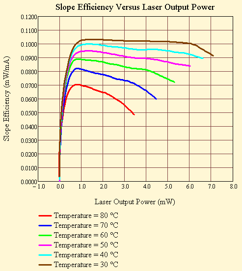
Note that Equation 1 shows SE as a function of IDrive and temperature. However, I need to relate SE (the derivative of POutput) to POutput. All I need to do is to plot SE versus POutput by using IDrive as a parameter.

Analysis

My Data

Figure 1 shows a plot of the data I have. The data always comes to me in the form of an Excel worksheet, and it shows POutput versus IDrive at various temperatures. What I need is SE versus POutput at various temperatures.

Figure 1: Drive Current Versus Optical Power and Temperature

Figure 1: Drive Current Versus Optical Power and Temperature

Approach

Here is my approach for analyzing this data:

  • I insert an Excel component into Mathcad, and I then insert the data into the Excel component.
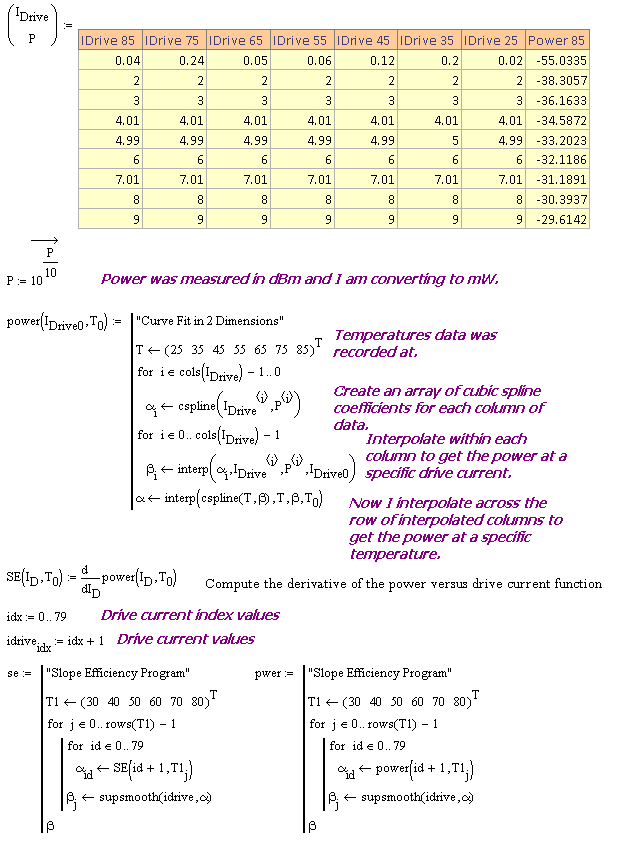
  • I perform a two-dimensional curve-fit using cubic splines to generate POutput(IDrive,T).
  • I compute SE by taking a derivative of POutput with respect to IDrive.
  • Compute POutput versus the same IDrive values that I used to compute SE.
  • I now plot my SE versus POutput for the same values of IDrive at various temperatures.

Interpolation

Figure 2 shows a screenshot from Mathcad of my data and interpolation approach. I used a Mathcad program to actually process the data. I find the programs simple to develop and easy to use.

Figure 2: Test Data Component and Interpolation Programs.

Figure 2: Test Data Component and Interpolation Programs.

Slope Efficiency Versus Optical Power at Various Temperatures

Figure 3 shows the final result of my work. Note how SE degrades with temperature.

Figure 3: Slope Efficiency Versus Optical Power at Various Temperatures.

Figure 3: Slope Efficiency Versus Optical Power at Various Temperatures.

Figure 3: Laser Tracking Error Versus Temperature.

Conclusion

I thought this was a good, practical example illustrating two-dimensional interpolation applied in an actual application. I often need to present data in a way that differs from how the data was originally gathered. Interpolation allows me to obtain the data I need with minimal effort.

Posted in Electronics, Fiber Optics | Tagged | 4 Comments

Laser Tracking Error and Curve Fitting

Introduction

I had a request for an example of how the output power of a laser varies with temperature. We call this parameter tracking error. Tracking error varies from part to part and the manufacturers simply put a bound on this variation (e.g. ±1.5 dB). The variation is a function of temperature, but the variation is not consistent between parts.

The specific request I received was to provide an example of a part's tracking error for temperatures above room temperature. I have monitor current versus optical power and temperature data, and I need optical power versus temperature at fixed monitor currents. I ended up using Mathcad to beat my data into a form that makes generating plots easy.

This post will assume some knowledge of the electrical characteristics of a laser, which I covered in this post.

Background

Optical communication systems assume that the light power coupled onto a fiber from laser's front facet and the light emitted from the laser's rear facet (and measured by the monitor photodiode) are linearly related. Tracking error is a measure of the maximum deviation of this relationship from linearity. These deviations are primarily due to mismatches in the thermal coefficient of expansion for the materials that make up the optical modules. In order to plot tracking error versus temperature, we need to precisely define what tracking error is. Equation 1 presents the formal definition.

Eq. 1 \displaystyle \text{Tracking Error }={{\left. \max \left( 10\cdot \log \left( \frac{{{P}_{Output}}\left( T \right)}{{{P}_{Output}}\left( 25{}^\circ C \right)} \right) \right) \right|}_{{{I}_{Monitor}}\text{ constant}}}

where

  • POutput is the laser output power
  • T is the ambient temperature that is varying over a range from -40 °C to 85 °C
  • IMonitor, the current from the monitor photodiode, is held at a constant value.

Tracking error is the largest source of variation that we see in a laser's output power. It is also not predictable in any way that I have seen -- you cannot compensate for it like other temperature-dependent parameters.

Analysis

My Data

Our laser power feedback control systems work by maintaining a constant average monitor current over temperature. Figure 1 shows a plot of the data I have. The data always comes to me in the form of an Excel worksheet, and it shows monitor current versus optical power at various temperatures. What I need is optical power versus temperature at a fixed monitor current.

Figure 1: Monitor Current Versus Optical Power and Temperature.

Figure 1: Monitor Current Versus Optical Power and Temperature.

Approach

Here is my approach for analyzing this data:

  • I insert an Excel component into Mathcad and insert the data into the Excel component.
  • I perform a two-dimensional curve-fit using cubic splines.
  • I now plot my output power versus temperature for various monitor currents.

Interpolation

Figure 2 shows a screenshot from Mathcad of my data and interpolation approach. I used a Mathcad program to actually process the data. I find the programs simple to develop and easy to use.

Figure 2: Test Data Component and Interpolation Program.

Figure 2: Test Data Component and Interpolation Program.

Optical Power Versus Temperature at Fixed Monitor Currents

Figure 3 shows the final result of my work. While the plot is boring, it is what I needed to answer the question.

Figure 3: Laser Tracking Error Versus Temperature.

Figure 3: Laser Tracking Error Versus Temperature.

Conclusion

I thought this was a good, practical example illustrating two-dimensional interpolation applied in an actual application. I often need to present data in a way that differs from how the data was originally gathered. Interpolation allows me to obtain the data I need with minimal effort.

Posted in Electronics, Fiber Optics | Tagged | Comments Off on Laser Tracking Error and Curve Fitting

Non-UN Participants in the Olympics

I was listening to the radio today and I heard a reporter say that 205 countries were participating in the Olympics. I checked and that number is correct. That seemed like a lot of countries, so I went to the UN web site and they say that their are 193 countries in the UN. What is the difference between the two lists?

To find out, I grabbed the lists of Olympic and UN countries from the Olympic and UN web sites, threw them in Excel, and found the differences. It turns out that all UN-member countries are sending a athletes to the Olympics. But there are 12 Olympic participants that are not in the UN. Table 1 shows the list. I was not able to find explanations behind their being granted independent Olympic status.

Table 1: Non-UN Participants in the Olympics
American Samoa
Aruba
Bermuda
British Virgin Islands
Cayman Islands
Republic of the Cook Islands
Guam
Hong Kong
Palestine (Not a UN member, but has observer status)
Puerto Rico
Taiwan (Chinese Taipei)
Virgin Islands
Posted in Personal | 4 Comments

Volcano Math

I was listening to Planetary Radio the other night and they had an interesting interview with Rosaly Lopes, a researcher at the Jet Propulsion Laboratory who has discovered more volcanoes than anyone else. Her discoveries were of volcanoes on other planets and satellites. This interview got me thinking -- just how many active volcanoes are there on Earth and where are they? This looks like a good job for Excel and pivot tables.

Time to go to the web and start hunting around. Very quickly I encountered a number of web sites (e.g. here and here) with lists of "active" volcanoes. Depending on your definition of active volcano, I have found sites that list between 400 and 1500 items. For no particular reason, I ended up focusing on the Volcano World web site from Oregon State University. They have a list of 430 volcanoes that was easy to import into Excel and will give me a feel for the number of volcanoes and where they are. Once the list is in Excel, we can start to ask questions about the data and get some answers.

One other quick point -- we have not discovered all of the volcanoes yet. For example, you occasionally hear of a previously unknown underwater volcano being discovered. So these lists do change occasionally. Also, the lists sometimes combine two nearby volcanoes in a single entry, like Tanaga and Takawangha. So you may see different numbers of volcanoes on different lists.

My question was about the number and location of the volcanoes. I also want to know what countries have the most volcanoes. I used a pivot table to divide the volcanoes up by country. Table 1 shows the results.

Table 1: Summary of Volcano Counts By Country.
Country Volcano Count
USA 81
Russia 55
Indonesia 45
Japan 40
Papua New Guinea 17
Ecuador 12
Philippines 11
Nicaragua 9
Ethiopia 9
Vanuatu 9
Chile 8
New Zealand 8
Kenya 7
Mexico 7
Guatemala 7
Italy 6
El Salvador 5
Greece 5
Spain 5
Iceland 5
Costa Rica 4
Australia 4
France 4
United Kingdom 4
Mariana Islands 4
Colombia 3
Tanzania 3
Portugal 3
Eritrea 2
Netherlands 2
Pacific Ocean 2
Peru 2
India 2
Cape Verde Islands 2
St. Kitts and Nevis 2
Philippines 2
Turkey 2
Democratic Republic of Congo 2
Cameroon 2
Azores (Portugal) 2
Solomon Islands 2
Iran 2
Ethiopia,Kenya 1
South Atlantic Ocean 1
Multiple Countries 1
Norway 1
Libya 1
Congo/Rwanda 1
Canary Islands (Spain) 1
Argentina 1
Comoros 1
Chad 1
Lesser Sunda Islands 1
Azores 1
St. Vincent 1
Antarctica 1
Tonga 1
Chile/Argentina 1
Uganda 1
Chile/Bolivia 1
Galápagos Islands 1
Rwanda, Congo 1
Grenada 1
China 1
Grand Total 430

I was surprised that the US had so many volcanoes. Let's take a closer look at the volcano count in the US by state. Just out of curiosity, I will separate out the Aleutian Islands from Alaska so that I can see where the volcanoes are in that area. Table 2 shows this data.

Table 2: Summary of Volcano Counts By State and Islands.
State/Region Volcano Count
Alaska 21
Aleutian Islands 18
Oregon 14
Hawaiian Islands 7
Washington 5
California 4
Arizona 4
Other Pacific Islands 2
Wyoming 2
New Mexico 2
Idaho 2
Grand Total 81

Now I want to look at the distribution percentage of volcanoes by state. I will recombine the Aleutians with Alaska. I will list non-state volcanoes in the "other Pacific Islands" category (e.g. Guguan and Pagan Islands). Table 3 shows this data.

Table 3: Summary of Volcano Percentages By State and Islands.
State/Region Volcano Percentage
Alaska and Aleutians 48.15%
Oregon 17.28%
Hawaiian Islands 8.64%
Washington 6.17%
California 4.94%
Arizona 4.94%
Other Pacific Islands 2.47%
Wyoming 2.47%
Idaho 2.47%
New Mexico 2.47%
Grand Total 100.00%

So nearly half of the US volcanoes are in Alaska and the Aleutians.

What I learned here was that the US has many more volcanoes than I would have thought and nearly half of them are in Alaska. I also showed that pivot tables are great for slicing up data like this.

Posted in General Science, software | Tagged , | 4 Comments

Lighting My House Number and Designing with Phototransistors

Introduction

I have had several people say that my house number is difficult to read at night. The number consists of four digits mounted on a structural column that holds up a section of my roof. In response to these complaints, my wife has asked that we install some sort of light for our house number. She was thinking we get someone like Aardvark Electric, Inc. (for light fixture installation) to do it but I thought it would make for an excellent project and blog post. Plus the structural column was rotting and needed to be replaced, I decided that it was a good time to replace the column as well whilst I lit up the house number.

Unfortunately, I could not find a light fixture that she liked, so I decided to build one from scratch. This blog post is about how I built the light. This was not a huge project, but it did involve me learning a bit about designing with phototransistors.

Requirements

My requirements are simple:

  • All wiring is low-voltage.

    I do not like running AC outdoors. I do not need an AC circuit to power a few LEDs.

  • I want the house numbers lit directly -- no side lighting.

    Some quick experiments showed that side lighting creates nasty shadows that makes the numbers hard to read.

  • The light enclosure must be made of cedar.

    This requirement comes from my wife. The structural column was not pretty. On the prompting of my wife, I clad the column in cedar. My wife likes the cedar and she was wondering if I could make the light enclosure out of cedar.

  • I will not use any cadmium.

    When I was a boy, I would have used a cadmium sulfide cell to sense the light level. Today, the toxicity of cadmium is well known and it is banned from any electronics that I design today. I take "green" design very seriously.

  • I will use LEDs for lighting.

    I like LEDs because they are energy efficient, run cool and I do not want anything hot in a cedar box. Even Neon Lights you see for a shop front or christmas decoration uses LEDs these days. If I need to install or replace any more lights in future I know what type to get.

  • I am only building one unit.

    Designing for production requires more than a weekend, which is all the time I have.

  • The light will turn on at sundown and off at sunup.

    The light is not needed during the day. We need to define what we mean by the light level at sundown and sunup. The Wikipedia describes the sunup/sundown light level as 400 lux. The lux is a photometric unit, which means it is defined with respect to the effect of electromagnetic radiation on the human eye. The sensitivity of the human eye varies with the wavelength of the light it is looking at. 400 lux corresponds to 585.6 mW/m at 555 nm. Sunlight has a nominal wavelength of 500 nm. Using the chart shown on this web page, we can see that the eye's sensitivity at 500 nm is pretty close to its sensitivity at 555 nm. So I will assume that sunlight at 400 lux can be modeled using a light power density of 585.6 mW/m at 500 nm. The results will be close enough.

Finished Project

Rather than wait until the end of this post, I will show you how everything ended up. Figure 1 shows the final product. Remember -- I am an amateur woodworker who threw this together on a weekend. However, my wife likes it and that is good enough for me.

Figure 1: My Light with Annotations.

Figure 1: My Light with Annotations.

Circuit Design

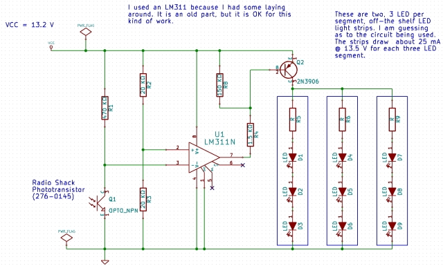
Figure 2 shows the circuit, which I captured in Kicad -- an open-source schematic/PCB layout tool. I used a simple comparator circuit to turn the light on at night. During daytime, the phototransistor is conducting, the comparator output is high, and the LEDs are off. When it is dark, the phototransistor is not conducting and the comparator output is low and the LEDs are on.

Figure 2: Schematic of My Light Sensor.

Figure 2: Schematic of My Light Sensor.

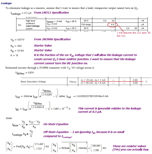
If I had more time, I would have added some hysteresis to the circuit. However, I am seeing no issues at this point, and I will just leave the circuit as it is. For the details on how I determined the values of R4 and R8, see Appendix A.

Project Design Elements

Mechanical Design

I designed the enclosure using Solidworks. This link provides an eDrawing of my design. Most folks do not have an eDrawing reader installed, but this reader is becoming the "Adobe Reader" of 3D mechanical design. I have a translucent plastic cover over the lamp that diffuses the light and ensures that we do not have to gaze upon bright LEDs. I found my plastic cover here , and I was amazed at all the options available.

Light Source

I started my project by looking for some LED strip lightning. Figure 3 shows a sample of the different kinds of strip lighting that I found. I chose the SMD3528, which I have enclosed in a red rectangle in Figure 3.

Figure 3: LED Strip Lighting Examples.

Figure 3: LED Strip Lighting Examples.

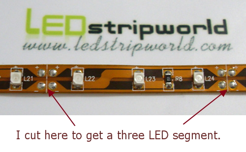
Figure 4 shows a closeup of the LED light strip that I bought.

Figure 4: Closeup of the Strip Lighting that I Finally Bought.

Figure 4: Closeup of the Strip Lighting that I Finally Bought.

Figure 5 shows the only specifications that I could find for the LED strip.

Figure 5: Specifications for the SMD3528 LED Strip.

Figure 5: Specifications for the SMD3528 LED Strip.

As shown in Figure 5, the strips are specified to draw 20 mA per 3 LED segment. I actually measured 25 mA per 3 LED segment.

Phototransistor

Specifications

A phototransistor is basically a transistor with a package that allows light of some wavelength to penetrate right down to the silicon. It turns out that many transistors are light-sensitive. I have even heard of people exposing the die of a 2N2222 transistor and using that as a phototransistor. One common difference from a normal three-terminal device is that many phototransistors only have two terminals (emitter and collector) because the light generates the base current. There are three-terminal phototransistors and they allow you to connect up a base resistor to control the sensitivity of the device. I only had a two-terminal phototransistor laying around.

I have some Radio Shack parts laying around the house, including a phototransistor (RS Part Number 276-0145). The only specifications I could find for this part were on the web and are shown in Figure 6.

Figure 6: Rough Specification for the Radio Shack 276-0145 Phototransistor

Figure 6: Rough Specification for the Radio Shack 276-0145 Phototransistor

From a design standpoint, the key specification is for the "light current," which is a parameter that relates collector current to the incident light power density.

Eq. 1 I_C={\gamma_{880nm}}\cdot S_{500nm/880nm}\cdot {{P}_{Light}}+{{I}_{Dark}}

where

  • IC is the phototransistor collector current (in mA).
  • PLight is the input optical power level @ 500nm (= 585.6 mW/cm ).
  • γ880nm is the collector current to light power density level (=20 mA/(20 mW/m ) @ 880 nm - my assumed wavelength of maximum sensitivity for an infrared phototransistor).
  • S500nm/880nm is the sensitivity correction from the phototransistor's reference level to the average sunlight wavelength of 500 nm (= 17%, Figure 7).
  • IDark is the phototransistor dark current (100 nA, specification).

Phototransistor Sensitivity Versus Wavelength

The Radio Shack phototransistor is target for infrared applications, like television remotes. However, these phototransistors can detect visible light, albeit with less sensitivity than infrared light. Unfortunately, the Radio Shack part specification does not state its sensitivity as a function of wavelength. I found a specification for a similar part from Vishay (BPV11) that does include this information. Figure 9 shows the BPV11's sensitivity versus wavelength and I will assume the Radio Shack phototransistor has the same wavelength dependence.

Figure 7: BPV11 Phototransistor Sensitivity Versus Wavelength.

Figure 7: BPV11 Phototransistor Sensitivity Versus Light Wavelength.

I now have enough information to complete the design the circuit.

Selection of Resistor R1

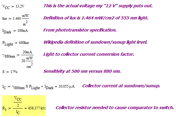
The only component that requires some design work is R1 (see Figure 1). I have set the comparator to trigger when the voltage drop across R1 is one half the supply voltage (= 13.2 V/2 = 6.6 V). The calculation is shown in Figure 8.

Figure 8: Calculation of R1 Value.

Figure 8: Calculation of R1 Value.

The ideal value for R1 would be 656 kΩ. I do not have that resistor value laying around, but I do have 470 kΩ. While a little low in value, it just means that light will turn off and on when it is a bit lighter out than 400 lux -- no big deal.

Conclusion

I built the circuit and it turns on at sunset (9:00 PM at 45 latitude one week after the summer solstice). My wife is happy -- I am happy.

Appendix A:Calculation of R4 and R8

Figure 9 shows how I derived the resistor values for driving transistor Q2.

Figure 9: R4 and R8 Resistor Value Derivations.

Figure 9: R4 and R8 Resistor Value Derivations.

Posted in Construction, Electronics | Tagged | 5 Comments