Heating a Room with People

I am currently sitting in a really boring meeting that is being held in a very small room. The room is packed full of people and it is hot in here. Of course, there is a part of me that is glad that the room is hot because I would hate for it to be too cold. I hate being cold, and if it goes on to affect my concentration, then I definitely won't be a happy bunny. My friend found himself in the same situation not so long ago. His boiler had decided to break on him and he was subsequently left with no heating and no hot water, which as you can imagine, was a complete nightmare for him. It wasn't until he was pointed in the direction of somewhere like this gas boiler service Durham company that he was able to get warm again. Thank goodness because I'm not sure how he would've coped otherwise.

So, after all of that, you could definitely say that the heater in the room that we were in was definitely working. Maybe it was too warm... All the same, I'm just glad that we weren't freezing cold. After thinking about it though, this situation reminds me of a conversation I had with a Universal HVAC services engineer many years ago about the heat load that people present to a cooling system. During that discussion, the HVAC engineer casually mentioned that he models every person as a 100 W load. I should be able to estimate that number based on the average daily calorie consumption of a person. Consider the calculation I show in Equation 1.

Eq. 1 \displaystyle P=\frac{E}{T}=\frac{2000\text{ kcalorie}}{24\text{ hours}}\cdot \frac{1\text{ hour}}{3600\text{ seconds}}\cdot \frac{4187\text{ Joules}}{\text{kcalorie}}=96.9 \text{ W}

where

The use of 100 W per person seems like a reasonable average number.

Posted in Construction | 3 Comments

Laser Slope Efficiency and Curve Fitting

Introduction

I have spent much of my summer dealing with issues related to the high temperature characteristics of lasers. These issues have stirred within me an interest in laser slope efficiency . Slope efficiency, also known as SE, is simply the slope of the laser's output power versus drive current curve. It varies from part-to-part and with temperature.

I am interested in how SE changes at temperatures above room temperature, which I will define here as 25 °C. I have drive current versus optical power and temperature data, and I need slope efficiency versus optical power at various temperature levels. This means more hammering of data into the form that I need for presentation.

This post will assume some knowledge of the electrical characteristics of a laser, which I covered in this post.

Background

If I had my choice, I would make SE a constant. Unfortunately, nature has not been that kind. As with most things electronic, things degrade rapidly with increasing temperature. In order to plot SE versus optical power at various temperatures, we need to precisely define what SE is. Equation 1 presents the formal definition.

Eq. 1 \displaystyle SE=\frac{d{{P}_{Output}}\left( {{I}_{Drive}},T \right)}{d{{I}_{Drive}}}

where

  • POutput is the laser output power, which is a function of drive current and temperature
  • T is the ambient temperature that is varying over a range from 30 °C to 80 °C
  • IDrive, the drive current into the laser.

Note that Equation 1 shows SE as a function of IDrive and temperature. However, I need to relate SE (the derivative of POutput) to POutput. All I need to do is to plot SE versus POutput by using IDrive as a parameter.

Analysis

My Data

Figure 1 shows a plot of the data I have. The data always comes to me in the form of an Excel worksheet, and it shows POutput versus IDrive at various temperatures. What I need is SE versus POutput at various temperatures.

Figure 1: Drive Current Versus Optical Power and Temperature

Figure 1: Drive Current Versus Optical Power and Temperature

Approach

Here is my approach for analyzing this data:

  • I insert an Excel component into Mathcad, and I then insert the data into the Excel component.
  • I perform a two-dimensional curve-fit using cubic splines to generate POutput(IDrive,T).
  • I compute SE by taking a derivative of POutput with respect to IDrive.
  • Compute POutput versus the same IDrive values that I used to compute SE.
  • I now plot my SE versus POutput for the same values of IDrive at various temperatures.

Interpolation

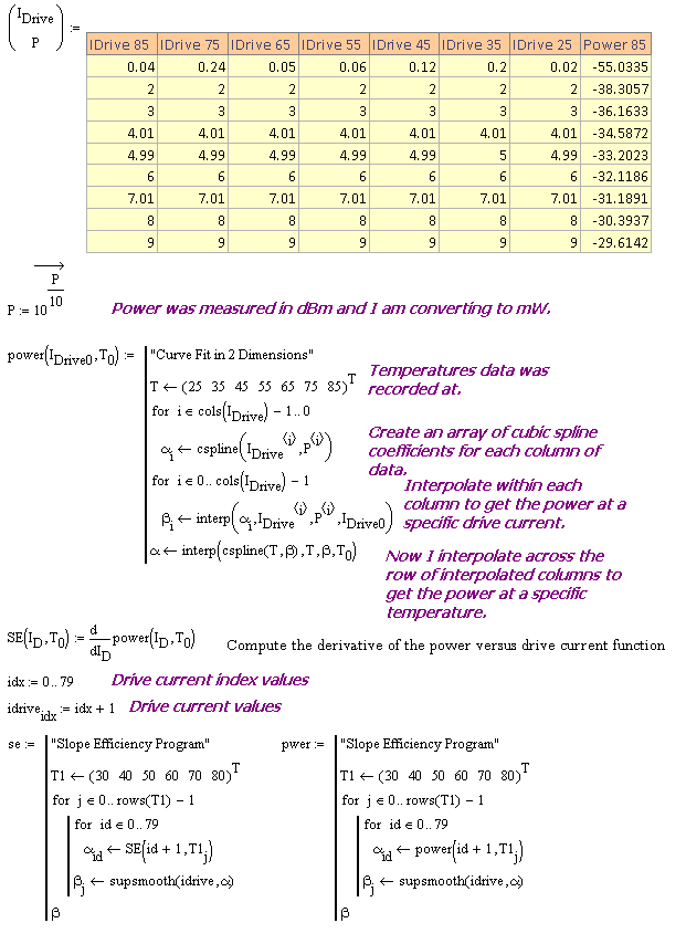
Figure 2 shows a screenshot from Mathcad of my data and interpolation approach. I used a Mathcad program to actually process the data. I find the programs simple to develop and easy to use.

Figure 2: Test Data Component and Interpolation Programs.

Figure 2: Test Data Component and Interpolation Programs.

Slope Efficiency Versus Optical Power at Various Temperatures

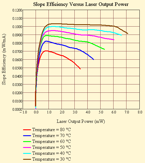
Figure 3 shows the final result of my work. Note how SE degrades with temperature.

Figure 3: Slope Efficiency Versus Optical Power at Various Temperatures.

Figure 3: Slope Efficiency Versus Optical Power at Various Temperatures.

Figure 3: Laser Tracking Error Versus Temperature.

Conclusion

I thought this was a good, practical example illustrating two-dimensional interpolation applied in an actual application. I often need to present data in a way that differs from how the data was originally gathered. Interpolation allows me to obtain the data I need with minimal effort.

Posted in Electronics, Fiber Optics | Tagged | 4 Comments

Laser Tracking Error and Curve Fitting

Introduction

I had a request for an example of how the output power of a laser varies with temperature. We call this parameter tracking error. Tracking error varies from part to part and the manufacturers simply put a bound on this variation (e.g. ±1.5 dB). The variation is a function of temperature, but the variation is not consistent between parts.

The specific request I received was to provide an example of a part's tracking error for temperatures above room temperature. I have monitor current versus optical power and temperature data, and I need optical power versus temperature at fixed monitor currents. I ended up using Mathcad to beat my data into a form that makes generating plots easy.

This post will assume some knowledge of the electrical characteristics of a laser, which I covered in this post.

Background

Optical communication systems assume that the light power coupled onto a fiber from laser's front facet and the light emitted from the laser's rear facet (and measured by the monitor photodiode) are linearly related. Tracking error is a measure of the maximum deviation of this relationship from linearity. These deviations are primarily due to mismatches in the thermal coefficient of expansion for the materials that make up the optical modules. In order to plot tracking error versus temperature, we need to precisely define what tracking error is. Equation 1 presents the formal definition.

Eq. 1 \displaystyle \text{Tracking Error }={{\left. \max \left( 10\cdot \log \left( \frac{{{P}_{Output}}\left( T \right)}{{{P}_{Output}}\left( 25{}^\circ C \right)} \right) \right) \right|}_{{{I}_{Monitor}}\text{ constant}}}

where

  • POutput is the laser output power
  • T is the ambient temperature that is varying over a range from -40 °C to 85 °C
  • IMonitor, the current from the monitor photodiode, is held at a constant value.

Tracking error is the largest source of variation that we see in a laser's output power. It is also not predictable in any way that I have seen -- you cannot compensate for it like other temperature-dependent parameters.

Analysis

My Data

Our laser power feedback control systems work by maintaining a constant average monitor current over temperature. Figure 1 shows a plot of the data I have. The data always comes to me in the form of an Excel worksheet, and it shows monitor current versus optical power at various temperatures. What I need is optical power versus temperature at a fixed monitor current.

Figure 1: Monitor Current Versus Optical Power and Temperature.

Figure 1: Monitor Current Versus Optical Power and Temperature.

Approach

Here is my approach for analyzing this data:

  • I insert an Excel component into Mathcad and insert the data into the Excel component.
  • I perform a two-dimensional curve-fit using cubic splines.
  • I now plot my output power versus temperature for various monitor currents.

Interpolation

Figure 2 shows a screenshot from Mathcad of my data and interpolation approach. I used a Mathcad program to actually process the data. I find the programs simple to develop and easy to use.

Figure 2: Test Data Component and Interpolation Program.

Figure 2: Test Data Component and Interpolation Program.

Optical Power Versus Temperature at Fixed Monitor Currents

Figure 3 shows the final result of my work. While the plot is boring, it is what I needed to answer the question.

Figure 3: Laser Tracking Error Versus Temperature.

Figure 3: Laser Tracking Error Versus Temperature.

Conclusion

I thought this was a good, practical example illustrating two-dimensional interpolation applied in an actual application. I often need to present data in a way that differs from how the data was originally gathered. Interpolation allows me to obtain the data I need with minimal effort.

Posted in Electronics, Fiber Optics | Tagged | Comments Off on Laser Tracking Error and Curve Fitting

Non-UN Participants in the Olympics

I was listening to the radio today and I heard a reporter say that 205 countries were participating in the Olympics. I checked and that number is correct. That seemed like a lot of countries, so I went to the UN web site and they say that their are 193 countries in the UN. What is the difference between the two lists?

To find out, I grabbed the lists of Olympic and UN countries from the Olympic and UN web sites, threw them in Excel, and found the differences. It turns out that all UN-member countries are sending a athletes to the Olympics. But there are 12 Olympic participants that are not in the UN. Table 1 shows the list. I was not able to find explanations behind their being granted independent Olympic status.

Table 1: Non-UN Participants in the Olympics
American Samoa
Aruba
Bermuda
British Virgin Islands
Cayman Islands
Republic of the Cook Islands
Guam
Hong Kong
Palestine (Not a UN member, but has observer status)
Puerto Rico
Taiwan (Chinese Taipei)
Virgin Islands
Posted in Personal | 4 Comments

Volcano Math

I was listening to Planetary Radio the other night and they had an interesting interview with Rosaly Lopes, a researcher at the Jet Propulsion Laboratory who has discovered more volcanoes than anyone else. Her discoveries were of volcanoes on other planets and satellites. This interview got me thinking -- just how many active volcanoes are there on Earth and where are they? This looks like a good job for Excel and pivot tables.

Time to go to the web and start hunting around. Very quickly I encountered a number of web sites (e.g. here and here) with lists of "active" volcanoes. Depending on your definition of active volcano, I have found sites that list between 400 and 1500 items. For no particular reason, I ended up focusing on the Volcano World web site from Oregon State University. They have a list of 430 volcanoes that was easy to import into Excel and will give me a feel for the number of volcanoes and where they are. Once the list is in Excel, we can start to ask questions about the data and get some answers.

One other quick point -- we have not discovered all of the volcanoes yet. For example, you occasionally hear of a previously unknown underwater volcano being discovered. So these lists do change occasionally. Also, the lists sometimes combine two nearby volcanoes in a single entry, like Tanaga and Takawangha. So you may see different numbers of volcanoes on different lists.

My question was about the number and location of the volcanoes. I also want to know what countries have the most volcanoes. I used a pivot table to divide the volcanoes up by country. Table 1 shows the results.

Table 1: Summary of Volcano Counts By Country.
Country Volcano Count
USA 81
Russia 55
Indonesia 45
Japan 40
Papua New Guinea 17
Ecuador 12
Philippines 11
Nicaragua 9
Ethiopia 9
Vanuatu 9
Chile 8
New Zealand 8
Kenya 7
Mexico 7
Guatemala 7
Italy 6
El Salvador 5
Greece 5
Spain 5
Iceland 5
Costa Rica 4
Australia 4
France 4
United Kingdom 4
Mariana Islands 4
Colombia 3
Tanzania 3
Portugal 3
Eritrea 2
Netherlands 2
Pacific Ocean 2
Peru 2
India 2
Cape Verde Islands 2
St. Kitts and Nevis 2
Philippines 2
Turkey 2
Democratic Republic of Congo 2
Cameroon 2
Azores (Portugal) 2
Solomon Islands 2
Iran 2
Ethiopia,Kenya 1
South Atlantic Ocean 1
Multiple Countries 1
Norway 1
Libya 1
Congo/Rwanda 1
Canary Islands (Spain) 1
Argentina 1
Comoros 1
Chad 1
Lesser Sunda Islands 1
Azores 1
St. Vincent 1
Antarctica 1
Tonga 1
Chile/Argentina 1
Uganda 1
Chile/Bolivia 1
Galápagos Islands 1
Rwanda, Congo 1
Grenada 1
China 1
Grand Total 430

I was surprised that the US had so many volcanoes. Let's take a closer look at the volcano count in the US by state. Just out of curiosity, I will separate out the Aleutian Islands from Alaska so that I can see where the volcanoes are in that area. Table 2 shows this data.

Table 2: Summary of Volcano Counts By State and Islands.
State/Region Volcano Count
Alaska 21
Aleutian Islands 18
Oregon 14
Hawaiian Islands 7
Washington 5
California 4
Arizona 4
Other Pacific Islands 2
Wyoming 2
New Mexico 2
Idaho 2
Grand Total 81

Now I want to look at the distribution percentage of volcanoes by state. I will recombine the Aleutians with Alaska. I will list non-state volcanoes in the "other Pacific Islands" category (e.g. Guguan and Pagan Islands). Table 3 shows this data.

Table 3: Summary of Volcano Percentages By State and Islands.
State/Region Volcano Percentage
Alaska and Aleutians 48.15%
Oregon 17.28%
Hawaiian Islands 8.64%
Washington 6.17%
California 4.94%
Arizona 4.94%
Other Pacific Islands 2.47%
Wyoming 2.47%
Idaho 2.47%
New Mexico 2.47%
Grand Total 100.00%

So nearly half of the US volcanoes are in Alaska and the Aleutians.

What I learned here was that the US has many more volcanoes than I would have thought and nearly half of them are in Alaska. I also showed that pivot tables are great for slicing up data like this.

Posted in General Science, software | Tagged , | 4 Comments

Lighting My House Number and Designing with Phototransistors

Introduction

I have had several people say that my house number is difficult to read at night. The number consists of four digits mounted on a structural column that holds up a section of my roof. In response to these complaints, my wife has asked that we install some sort of light for our house number. She was thinking we get someone like Aardvark Electric, Inc. (for light fixture installation) to do it but I thought it would make for an excellent project and blog post. Plus the structural column was rotting and needed to be replaced, I decided that it was a good time to replace the column as well whilst I lit up the house number.

Unfortunately, I could not find a light fixture that she liked, so I decided to build one from scratch. This blog post is about how I built the light. This was not a huge project, but it did involve me learning a bit about designing with phototransistors.

Requirements

My requirements are simple:

  • All wiring is low-voltage.

    I do not like running AC outdoors. I do not need an AC circuit to power a few LEDs.

  • I want the house numbers lit directly -- no side lighting.

    Some quick experiments showed that side lighting creates nasty shadows that makes the numbers hard to read.

  • The light enclosure must be made of cedar.

    This requirement comes from my wife. The structural column was not pretty. On the prompting of my wife, I clad the column in cedar. My wife likes the cedar and she was wondering if I could make the light enclosure out of cedar.

  • I will not use any cadmium.

    When I was a boy, I would have used a cadmium sulfide cell to sense the light level. Today, the toxicity of cadmium is well known and it is banned from any electronics that I design today. I take "green" design very seriously.

  • I will use LEDs for lighting.

    I like LEDs because they are energy efficient, run cool and I do not want anything hot in a cedar box. Even Neon Lights you see for a shop front or christmas decoration uses LEDs these days. If I need to install or replace any more lights in future I know what type to get.

  • I am only building one unit.

    Designing for production requires more than a weekend, which is all the time I have.

  • The light will turn on at sundown and off at sunup.

    The light is not needed during the day. We need to define what we mean by the light level at sundown and sunup. The Wikipedia describes the sunup/sundown light level as 400 lux. The lux is a photometric unit, which means it is defined with respect to the effect of electromagnetic radiation on the human eye. The sensitivity of the human eye varies with the wavelength of the light it is looking at. 400 lux corresponds to 585.6 mW/m at 555 nm. Sunlight has a nominal wavelength of 500 nm. Using the chart shown on this web page, we can see that the eye's sensitivity at 500 nm is pretty close to its sensitivity at 555 nm. So I will assume that sunlight at 400 lux can be modeled using a light power density of 585.6 mW/m at 500 nm. The results will be close enough.

Finished Project

Rather than wait until the end of this post, I will show you how everything ended up. Figure 1 shows the final product. Remember -- I am an amateur woodworker who threw this together on a weekend. However, my wife likes it and that is good enough for me.

Figure 1: My Light with Annotations.

Figure 1: My Light with Annotations.

Circuit Design

Figure 2 shows the circuit, which I captured in Kicad -- an open-source schematic/PCB layout tool. I used a simple comparator circuit to turn the light on at night. During daytime, the phototransistor is conducting, the comparator output is high, and the LEDs are off. When it is dark, the phototransistor is not conducting and the comparator output is low and the LEDs are on.
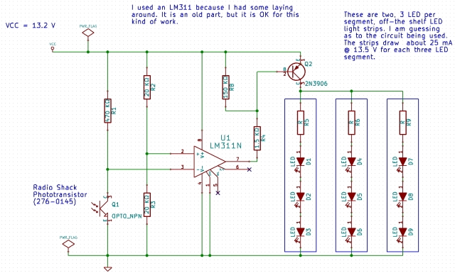
Figure 2: Schematic of My Light Sensor.

Figure 2: Schematic of My Light Sensor.

If I had more time, I would have added some hysteresis to the circuit. However, I am seeing no issues at this point, and I will just leave the circuit as it is. For the details on how I determined the values of R4 and R8, see Appendix A.

Project Design Elements

Mechanical Design

I designed the enclosure using Solidworks. This link provides an eDrawing of my design. Most folks do not have an eDrawing reader installed, but this reader is becoming the "Adobe Reader" of 3D mechanical design. I have a translucent plastic cover over the lamp that diffuses the light and ensures that we do not have to gaze upon bright LEDs. I found my plastic cover here , and I was amazed at all the options available.

Light Source

I started my project by looking for some LED strip lightning. Figure 3 shows a sample of the different kinds of strip lighting that I found. I chose the SMD3528, which I have enclosed in a red rectangle in Figure 3.

Figure 3: LED Strip Lighting Examples.

Figure 3: LED Strip Lighting Examples.

Figure 4 shows a closeup of the LED light strip that I bought.
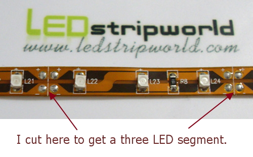
Figure 4: Closeup of the Strip Lighting that I Finally Bought.

Figure 4: Closeup of the Strip Lighting that I Finally Bought.

Figure 5 shows the only specifications that I could find for the LED strip.

Figure 5: Specifications for the SMD3528 LED Strip.

Figure 5: Specifications for the SMD3528 LED Strip.

As shown in Figure 5, the strips are specified to draw 20 mA per 3 LED segment. I actually measured 25 mA per 3 LED segment.

Phototransistor

Specifications

A phototransistor is basically a transistor with a package that allows light of some wavelength to penetrate right down to the silicon. It turns out that many transistors are light-sensitive. I have even heard of people exposing the die of a 2N2222 transistor and using that as a phototransistor. One common difference from a normal three-terminal device is that many phototransistors only have two terminals (emitter and collector) because the light generates the base current. There are three-terminal phototransistors and they allow you to connect up a base resistor to control the sensitivity of the device. I only had a two-terminal phototransistor laying around.

I have some Radio Shack parts laying around the house, including a phototransistor (RS Part Number 276-0145). The only specifications I could find for this part were on the web and are shown in Figure 6.

Figure 6: Rough Specification for the Radio Shack 276-0145 Phototransistor

Figure 6: Rough Specification for the Radio Shack 276-0145 Phototransistor

From a design standpoint, the key specification is for the "light current," which is a parameter that relates collector current to the incident light power density.

Eq. 1 I_C={\gamma_{880nm}}\cdot S_{500nm/880nm}\cdot {{P}_{Light}}+{{I}_{Dark}}

where

  • IC is the phototransistor collector current (in mA).
  • PLight is the input optical power level @ 500nm (= 585.6 mW/cm ).
  • γ880nm is the collector current to light power density level (=20 mA/(20 mW/m ) @ 880 nm - my assumed wavelength of maximum sensitivity for an infrared phototransistor).
  • S500nm/880nm is the sensitivity correction from the phototransistor's reference level to the average sunlight wavelength of 500 nm (= 17%, Figure 7).
  • IDark is the phototransistor dark current (100 nA, specification).

Phototransistor Sensitivity Versus Wavelength

The Radio Shack phototransistor is target for infrared applications, like television remotes. However, these phototransistors can detect visible light, albeit with less sensitivity than infrared light. Unfortunately, the Radio Shack part specification does not state its sensitivity as a function of wavelength. I found a specification for a similar part from Vishay (BPV11) that does include this information. Figure 9 shows the BPV11's sensitivity versus wavelength and I will assume the Radio Shack phototransistor has the same wavelength dependence.

Figure 7: BPV11 Phototransistor Sensitivity Versus Wavelength.

Figure 7: BPV11 Phototransistor Sensitivity Versus Light Wavelength.

I now have enough information to complete the design the circuit.

Selection of Resistor R1

The only component that requires some design work is R1 (see Figure 1). I have set the comparator to trigger when the voltage drop across R1 is one half the supply voltage (= 13.2 V/2 = 6.6 V). The calculation is shown in Figure 8.
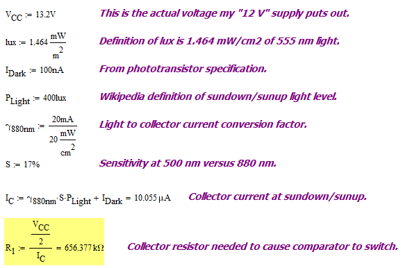
Figure 8: Calculation of R1 Value.

Figure 8: Calculation of R1 Value.

The ideal value for R1 would be 656 kΩ. I do not have that resistor value laying around, but I do have 470 kΩ. While a little low in value, it just means that light will turn off and on when it is a bit lighter out than 400 lux -- no big deal.

Conclusion

I built the circuit and it turns on at sunset (9:00 PM at 45 latitude one week after the summer solstice). My wife is happy -- I am happy.

Appendix A:Calculation of R4 and R8

Figure 9 shows how I derived the resistor values for driving transistor Q2.
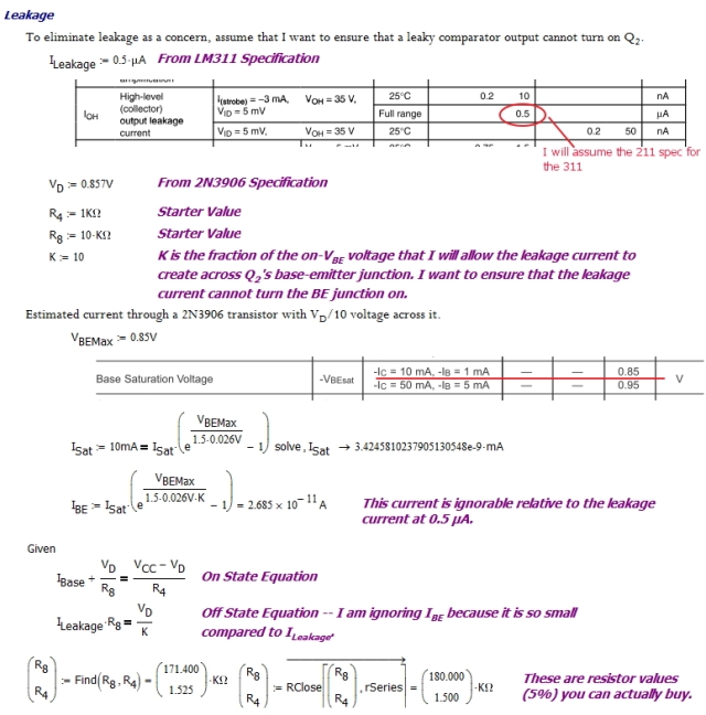
Figure 9: R4 and R8 Resistor Value Derivations.

Figure 9: R4 and R8 Resistor Value Derivations.
Posted in Construction, Electronics | Tagged | 5 Comments

Handling "Hot" Electronics Requires Gloves

I have had a number of equipment installers contact me this summer and express concerns about the temperature of the outdoor electronics that they are handling. In some cases, the electronics is too hot to hold. In every case, the temperatures of the products has been within specifications. I tell installers that a circuit card can be as hot as 95  °C and the components on it can be even hotter. Figure 1 illustrates the conditions that we design for. Note that the telecommunications industry often designs to Telcordia specifications, which are the basis of the temperature numbers that we use.

Figure 1: Telecommunications Outdoor Electronics Temperature Stackup.

Figure 1: Telecommunications Outdoor Electronics Temperature Stackup.

Figure 1 also mentions a commonly used junction temperature objective, which I discuss more here.

Figure 2 shows how hot something like this feels on human skin by showing burn time versus temperature (Source: "The Burn Wound", Chapter 1, Barret and Dziewulski).

Figure 2:Skin surface temperature needed to produce full thickness damage versus time.

Figure 2:Skin surface temperature needed to produce full thickness damage versus time.

So touching something that is at a temperature of 95 °C will cause a burn very quickly – it is just 5 °C less than the temperature of boiling water.

Personally, I always wear gloves.

Appendix

I have an objective of limiting the junction temperatures of parts in my designs to no more than 110 °C. I cannot always meet that objective. The US Navy set that junction temperature as an objective years ago in its reliability guidelines and is commonly used to this day in the design of electronic gear rated for outdoor use. Here is an example from the datasheet of the Cree SMD LED, which uses 110 °C as its maximum junction temperature.

Figure 2: Example of the use of 110 °C maximum.

Figure 2: Example of the Use of 110 °C Junction Temperature Maximum.

Posted in Electronics | Tagged , | 2 Comments

Some Empirical Potentiometer Results

Just a note that I have added some empirical test results to the following three posts on potentiometers.

Posted in Electronics | Comments Off on Some Empirical Potentiometer Results

Cost of Cooling Electronics

Introduction

One of my favorite physicists stopped by today and wanted to talk about the cost of cooling electronics like fans and air conditioners. The talk was somewhat mathematical and worth discussing here because the basic math is what a homeowner should do when evaluating the cost of different air conditioning options. In fact, my son recently chose an air conditioner based on this same calculation.

Problem Statement

The following problem statement pretty closely mirrors what I was asked today. I have omitted a few details having to do with the particular hardware chosen.

I have a customer who wants to add 200 Watts of electronics to an air-conditioned electronic enclosure. How much more will this customer's cooling costs increase each year when he adds this hardware to his enclosure?

Seems like a simple question and it is. Let's dig in ...

Approach

My approach to solving this problem is as follows.

  • Determine the total amount of power you are adding to the electronic enclosure.

    Most of the time you need to add up all the power dissipations and also add the cost of power conversion that may be involved. For example, telecommunications gear is often powered by 48 V gear. This means that the total power dissipation will include the power dissipated from the 48 V supply and the power dissipated when converting the building power (AC) to 48 V. The conversion process is ~80% efficient. The exact number depends on the specific power converter you are using.The total power dissipated, including conversion losses, is given by the equation PTotalThermal = PThermal/kEfficiency, where PThermal is the power dissipated within the telecommunications gear, PTotalThermal is PThermal plus conversion losses, and kEfficiency is the conversion efficiency.

  • Convert the electrical power from Watts to BTUs.

    I live in the US. Unit conversion is a part of life.

  • Use the Seasonal Energy Efficiency Ration (SEER) to convert BTUs of cooling to electrical power in kilo-Watts (kW).

    SEER is a conversion factor that air conditioner manufacturers are required to state. The Wikipedia has an excellent discussion on SEER and you should go there for more information.

  • Compute the yearly energy usage.

    Just multiply the Watts dissipated times the total number of hours in a year to get Watt-hours, which can then be converted to kW-hours.

  • Convert kW to dollars using the local cost of electricity.

    The US Department of Energy (DoE) publishes the average cost of electricity in every state. I have a blog post that presents this data in graphic form.

Analysis

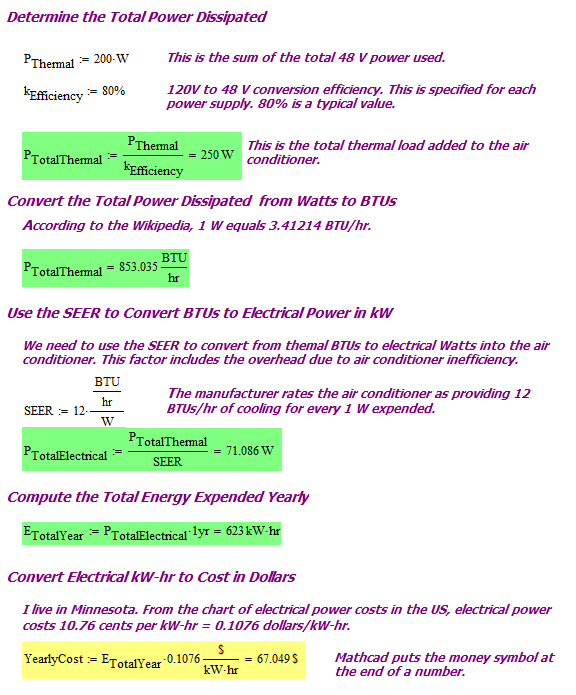
Figure 1 summarizes my analysis in Mathcad.

Figure 1: Analysis of the Yearly Airconditioning Cost Increment

Figure 1: Analysis of the Yearly Airconditioning Cost Increment


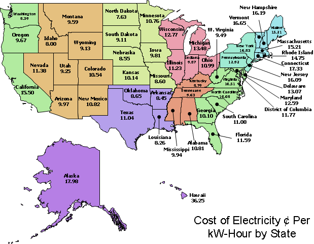
Figure 2 repeats my graph of electrical costs in the US from this blog post.
Figure 2: Electrical Power Costs in the US.

Figure 2: Electrical Power Costs in the US.

Conclusion

The customer is going to burn more than $67 every year just to power the air conditioner for this hardware. Of course this is assuming they have HVAC repair at regular intervals. The cost will only go up the longer the air conditioner units have gone without cleaning or servicing. Thus, understanding the need of a timely inspection of an HVAC unit by a professional similar to ac services Douglas County (or similar others) is of utmost importance. The cost may only go down if the customer finds a more efficient conditioner than the one they're currently using on the market, but now we're just getting into hypotheticals.

To get the total electrical cost, the customer will need to add the cost of powering the electronics itself. This is all part of the cost of doing business I suppose.

Posted in Construction, Electronics | Comments Off on Cost of Cooling Electronics

Yet Another Circuit with a "Logarithmic" Characteristic

Introduction

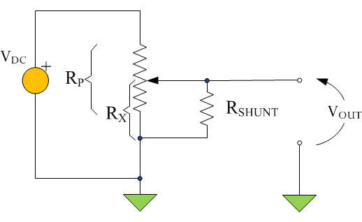
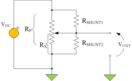
While I was looking for different circuits that generate a logarithmic characteristic (voltage, current, or resistance), I stumbled upon a web page that discussed a logarithmic potentiometer approximation using a linear potentiometer with one or two resistors connected to the wiper as shown in Figures 1 and 2. Note that this potentiometer characteristic is actually exponential -- why this nomenclature inconsistency has developed is beyond me.

Figure 1: Logarithmic Approximation Using a Single Resistor Across the Wiper.

Figure 1: Logarithmic Approximation Using a Single Resistor Across the Wiper.

Figure 2: Logarithmic Approximation Using Two Resistors Connected to the Wiper.

Figure 2: Logarithmic Approximation Using Two Resistors Connected to the Wiper.

As I continued hunting, I found an excellent article that describes creating a Verilog model for the same circuit using Qucs  (a circuit simulator that I like).

My goal here is to create a circuit that produces an output voltage that is related approximately to a exponential function with the wiper position as the argument (wiper position is expressed as a percentage of its full scale movement). My plan here is to use Mathcad to pick values for the resistors in both circuits that minimizes the maximum error of the logarithmic approximation.

One-Resistor Version

Figure 3 shows the results of my analysis of Figure 1. There is nothing special here as far as analysis goes. The results do indicate that the one-resistor circuit of Figure 1 produces a relatively poor result.

Figure 3: Setup and Calculation of Optimum Single Resistor Approximation.

Figure 3: Setup and Calculation of Optimum Single Resistor Approximation.

Two-Resistor Version

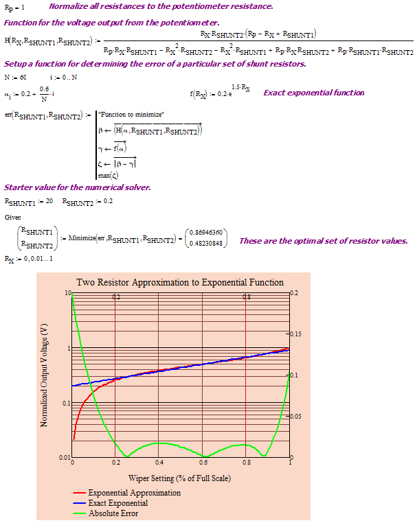
Figure 4 shows the results of my analysis of Figure 2. The results indicate that the two-resistor circuit of Figure 2 produces a relatively good result for wiper positions of 20% to 80%. I could see me using this approximation for some applications.

Figure 4: Setup and Calculation of Optimum Single Resistor Approximation.

Figure 4: Setup and Calculation of Optimum Single Resistor Approximation.

Conclusion

I included this post for completeness. I wanted to store away all the exponential circuit approximations that I found into a searchable database. See the Appendix for empirical results.

Appendix

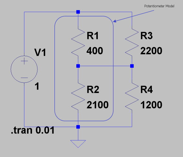
Figure 5 shows the circuit as I have it in LT Spice.

Figure 5: Circuit as Tested in Spice.

Figure 5: Circuit as Tested in Spice.


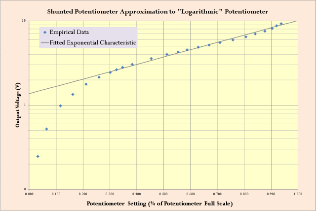
Figure 6 shows the empirical test data. Not too bad.
Figure 6: Empirical Test Data.

Figure 6: Empirical Test Data.

Posted in Electronics | Tagged | 1 Comment