Handling "Hot" Electronics Requires Gloves

I have had a number of equipment installers contact me this summer and express concerns about the temperature of the outdoor electronics that they are handling. In some cases, the electronics is too hot to hold. In every case, the temperatures of the products has been within specifications. I tell installers that a circuit card can be as hot as 95  °C and the components on it can be even hotter. Figure 1 illustrates the conditions that we design for. Note that the telecommunications industry often designs to Telcordia specifications, which are the basis of the temperature numbers that we use.

Figure 1: Telecommunications Outdoor Electronics Temperature Stackup.

Figure 1: Telecommunications Outdoor Electronics Temperature Stackup.

Figure 1 also mentions a commonly used junction temperature objective, which I discuss more here.

Figure 2 shows how hot something like this feels on human skin by showing burn time versus temperature (Source: "The Burn Wound", Chapter 1, Barret and Dziewulski).

Figure 2:Skin surface temperature needed to produce full thickness damage versus time.

Figure 2:Skin surface temperature needed to produce full thickness damage versus time.

So touching something that is at a temperature of 95 °C will cause a burn very quickly – it is just 5 °C less than the temperature of boiling water.

Personally, I always wear gloves.

Appendix

I have an objective of limiting the junction temperatures of parts in my designs to no more than 110 °C. I cannot always meet that objective. The US Navy set that junction temperature as an objective years ago in its reliability guidelines and is commonly used to this day in the design of electronic gear rated for outdoor use. Here is an example from the datasheet of the Cree SMD LED, which uses 110 °C as its maximum junction temperature.

Figure 2: Example of the use of 110 °C maximum.

Figure 2: Example of the Use of 110 °C Junction Temperature Maximum.

Posted in Electronics | Tagged , | 2 Comments

Some Empirical Potentiometer Results

Just a note that I have added some empirical test results to the following three posts on potentiometers.

Posted in Electronics | Comments Off on Some Empirical Potentiometer Results

Cost of Cooling Electronics

Introduction

One of my favorite physicists stopped by today and wanted to talk about the cost of cooling electronics like fans and air conditioners. The talk was somewhat mathematical and worth discussing here because the basic math is what a homeowner should do when evaluating the cost of different air conditioning options. In fact, my son recently chose an air conditioner based on this same calculation.

Problem Statement

The following problem statement pretty closely mirrors what I was asked today. I have omitted a few details having to do with the particular hardware chosen.

I have a customer who wants to add 200 Watts of electronics to an air-conditioned electronic enclosure. How much more will this customer's cooling costs increase each year when he adds this hardware to his enclosure?

Seems like a simple question and it is. Let's dig in ...

Approach

My approach to solving this problem is as follows.

  • Determine the total amount of power you are adding to the electronic enclosure.

    Most of the time you need to add up all the power dissipations and also add the cost of power conversion that may be involved. For example, telecommunications gear is often powered by 48 V gear. This means that the total power dissipation will include the power dissipated from the 48 V supply and the power dissipated when converting the building power (AC) to 48 V. The conversion process is ~80% efficient. The exact number depends on the specific power converter you are using.The total power dissipated, including conversion losses, is given by the equation PTotalThermal = PThermal/kEfficiency, where PThermal is the power dissipated within the telecommunications gear, PTotalThermal is PThermal plus conversion losses, and kEfficiency is the conversion efficiency.

  • Convert the electrical power from Watts to BTUs.

    I live in the US. Unit conversion is a part of life.

  • Use the Seasonal Energy Efficiency Ration (SEER) to convert BTUs of cooling to electrical power in kilo-Watts (kW).

    SEER is a conversion factor that air conditioner manufacturers are required to state. The Wikipedia has an excellent discussion on SEER and you should go there for more information.

  • Compute the yearly energy usage.

    Just multiply the Watts dissipated times the total number of hours in a year to get Watt-hours, which can then be converted to kW-hours.

  • Convert kW to dollars using the local cost of electricity.

    The US Department of Energy (DoE) publishes the average cost of electricity in every state. I have a blog post that presents this data in graphic form.

Analysis

Figure 1 summarizes my analysis in Mathcad.

Figure 1: Analysis of the Yearly Airconditioning Cost Increment

Figure 1: Analysis of the Yearly Airconditioning Cost Increment


Figure 2 repeats my graph of electrical costs in the US from this blog post.
Figure 2: Electrical Power Costs in the US.

Figure 2: Electrical Power Costs in the US.

Conclusion

The customer is going to burn more than $67 every year just to power the air conditioner for this hardware. Of course this is assuming they have HVAC repair at regular intervals. The cost will only go up the longer the air conditioner units have gone without cleaning or servicing. Thus, understanding the need of a timely inspection of an HVAC unit by a professional similar to ac services Douglas County (or similar others) is of utmost importance. The cost may only go down if the customer finds a more efficient conditioner than the one they're currently using on the market, but now we're just getting into hypotheticals.

To get the total electrical cost, the customer will need to add the cost of powering the electronics itself. This is all part of the cost of doing business I suppose.

Posted in Construction, Electronics | Comments Off on Cost of Cooling Electronics

Yet Another Circuit with a "Logarithmic" Characteristic

Introduction

While I was looking for different circuits that generate a logarithmic characteristic (voltage, current, or resistance), I stumbled upon a web page that discussed a logarithmic potentiometer approximation using a linear potentiometer with one or two resistors connected to the wiper as shown in Figures 1 and 2. Note that this potentiometer characteristic is actually exponential -- why this nomenclature inconsistency has developed is beyond me.

Figure 1: Logarithmic Approximation Using a Single Resistor Across the Wiper.

Figure 1: Logarithmic Approximation Using a Single Resistor Across the Wiper.

Figure 2: Logarithmic Approximation Using Two Resistors Connected to the Wiper.

Figure 2: Logarithmic Approximation Using Two Resistors Connected to the Wiper.

As I continued hunting, I found an excellent article that describes creating a Verilog model for the same circuit using Qucs  (a circuit simulator that I like).

My goal here is to create a circuit that produces an output voltage that is related approximately to a exponential function with the wiper position as the argument (wiper position is expressed as a percentage of its full scale movement). My plan here is to use Mathcad to pick values for the resistors in both circuits that minimizes the maximum error of the logarithmic approximation.

One-Resistor Version

Figure 3 shows the results of my analysis of Figure 1. There is nothing special here as far as analysis goes. The results do indicate that the one-resistor circuit of Figure 1 produces a relatively poor result.

Figure 3: Setup and Calculation of Optimum Single Resistor Approximation.

Figure 3: Setup and Calculation of Optimum Single Resistor Approximation.

Two-Resistor Version

Figure 4 shows the results of my analysis of Figure 2. The results indicate that the two-resistor circuit of Figure 2 produces a relatively good result for wiper positions of 20% to 80%. I could see me using this approximation for some applications.

Figure 4: Setup and Calculation of Optimum Single Resistor Approximation.

Figure 4: Setup and Calculation of Optimum Single Resistor Approximation.

Conclusion

I included this post for completeness. I wanted to store away all the exponential circuit approximations that I found into a searchable database. See the Appendix for empirical results.

Appendix

Figure 5 shows the circuit as I have it in LT Spice.

Figure 5: Circuit as Tested in Spice.

Figure 5: Circuit as Tested in Spice.


Figure 6 shows the empirical test data. Not too bad.
Figure 6: Empirical Test Data.

Figure 6: Empirical Test Data.

Posted in Electronics | Tagged | 1 Comment

Wall-Wart Math

I have had some questions recently on the power conversion efficiency of AC power adapters (aka "wall warts"). I think my customers are becoming more concerned about energy costs. The questions that I received focused on how the efficiency of a wall wart varies with how heavily it is loaded (load factor = actual load/maximum rated load). For example, a wall wart rated for 20 W but driving a 1 W load would be considered lightly loaded (load factor = 1 W/20 W = 5%). The same 20 W wall wart with a 20 watt load (load factor = 20 W/ 20 W= 100%) would be considered heavily loaded.

I did a quick search of the web and I could not find any conversion efficiency data for standard wall warts. Fortunately the measurements are simple, however there is one interesting aspect -- the input current is very non-linear. This means that I must do a numerical integration of the instantaneous power (= input current times input voltage) to determine the average power. This actually is simple because multiplying signals and integrating them are built-in features of today's oscilloscopes. Figure 1 shows an oscilloscope screenshot of the wall wart input voltage, current, and power.

Figure 1: Oscilloscope Screenshot of Wallwart AC Input Voltage, Current, and Power.

Figure 1: Oscilloscope Screenshot of Wallwart AC Input Voltage, Current, and Power.

Figure 2 contains my graph of the efficiency versus load factor (load factor = actual load/rated maximum load). For comparison, I added a plot of the efficiency of a very common UPS to the plots for the wall warts.

Figure 2: Wall Wart Efficiency Versus Load Factor.

Figure 2: Wall Wart Efficiency Versus Load Factor.


The plots show that wall warts have relatively constant conversion efficiency when loaded at 30% or higher.

Note:
Here is a discussion of wall-wart power conversion efficiency by the NRDC folks.

Posted in Electronics | 2 Comments

Product Feature Presentations Using Excel's AutoFilter and VBA

I have to present a lot of data to people, but I find PowerPoint, a corporate workhorse, to be a poor vehicle for presenting data. I am not an acolyte of Tufte -- a famous PowerPoint critic -- I just don't like PowerPoint presentations. Recently, I had to prepare a presentation on the cost of various options for a product. I decided that I wanted to create selectable product scenarios that would create a dynamic bill of material using Excel's AutoFilter feature. AutoFilter is a really useful feature, but it does not allow me to predefine scenarios. Here is where a bit of Visual Basic for Applications (VBA) helped out. This spreadsheet was easy to present to a room full of staff, and it allowed our Marketing and Systems folks to try out product feature options themselves and to see just how much different features cost.

The basic idea is simple:

  • create a bill of material with parts assigned to specific features (on tab called AutoFilter).
  • create lists of scenarios consisting of feature sets that make sense (on tab called Definitions)
  • assign the scenarios to radio buttons.

Here is my source workbook: Scenario Presenter

Posted in Management | Comments Off on Product Feature Presentations Using Excel's AutoFilter and VBA

Computer Museum in Bozeman Montana

I am currently in Bozeman, Montana, and I just took a tour of the "Museum of Modern Human Progress," formerly known as the American Computer Museum. I was with one of my sons, and the museum provided us a great opportunity to view the history of information and computing. One interesting item that was not highlighted much is their copy of the Antikythera mechanism, which was an early Greek computer. I have always found that device and its history interesting.

It was nice seeing some of the old computer hardware I worked on as a "wee lad." However, it does make me feel a tad old.

Posted in History of Science and Technology | Tagged | 4 Comments

Square Law Potentiometer Circuit

Quote of the Day

The question isn't who is going to let me; it's who is going to stop me.

— Ayn Rand


I do not have an immediate need for a circuit that generates an output voltage proportional to the square of the potentiometer setting, but this circuit was interesting enough that I thought I would document it here. I found it while looking for a logarithmic potentiometer circuit.

Figure 1 shows the original article describing the circuit.

Figure 1: Circuit that Generates a Square Law Voltage Output Based on a Potentiometer Setting.

Figure 1: Circuit that Generates a Square Law Voltage Output Based on a Potentiometer Setting.

This circuit generates an output voltage given by V_{OUT} = {{k}^{2}} \cdot V_{CC}, where k is the potentiometer setting as a percentage of full scale and VCC is the supply voltage.

To explain how this circuit works, let's redraw the circuit using idealized components (Figure 2).

Figure 2: Idealized Representation of the Circuit of Figure 1

Figure 2: Idealized Representation of the Circuit of Figure 1

For {{V}_{CC}}=I\cdot {{R}_{P}}, this circuit generates a voltage output of {{v}_{OUT}}={{k}^{2}}\cdot {{V}_{CC}}. Figure 3 shows my derivation.

Figure 3: Derivation of Square Law Characteristic.

Figure 3: Derivation of Square Law Characteristic.

There are lots of ways to build a current source that are well documented on the web, so I won't go into detail here. I will attach a Maxim reference that I think is excellent.
AN3869

Empirical Results

Figure 4 shows a version of this circuit that I simulated using LT Spice (free simulator).

Figure 4: Square Law Circuit From Simulator.

Figure 4: Square Law Circuit From Simulator.

Figure 5 shows my empirical data. I did no resistor tuning. Just threw it together and it seemed to work well.

Figure 5: Empirical Results.

Figure 5: Empirical Results.

Save

Posted in Electronics | 5 Comments

Another Circuit with a "Logarithmic" Characteristic

Introduction

Electronics is my profession and my hobby (along with mathematics). For a hobbyist project of mine, I need an amplifier circuit with a programmable gain that varies exponentially with the setting on a potentiometer. When I design a circuit, I usually begin my design effort with a web search. I do not like reinventing the wheel. I found an old EDN article that has an interesting circuit, but the figures are not visible. I will reconstruct the circuit here based on the text description and make a small modification that makes it a bit more appropriate for my application.

Note that this problem is closely related to an early post of mine on potentiometers. I could use a log potentiometer, which really have an exponential resistance characteristic, but I have not been satisfied with the accuracy and repeatability of these components. So I have looked for an alternative approach and this one seems reasonable.

Requirements

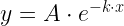
I need a circuit with a gain that varies exponentially according to the setting of a potentiometer. Equation 1 shows the functional form that I am looking for.

Eq. 1 y=A\cdot {{e}^{-k\cdot x}}

where

  • x is the potentiometer setting as a percentage of full-scale.
  • k is an arbitrary constant.
  • A is an arbitrary constant.

I often end up plotting my results on a semi-log plot. Equation 1 represents a straight line on a semi-log plot, which I prove in Equation 2.

Eq. 2 \ln \left( y \right)=-k\cdot x+b\Rightarrow y={{e}^{-k\cdot x+b}}
y={{e}^{-k\cdot x+b}}\Rightarrow y=A\cdot {{e}^{-k\cdot x}}\text{, where }A={{e}^{b}}

Knowing that Equation 1 will plot as a straight line will allow us to graph the circuit response and determine how well it conforms to Equation 1.

Original Circuit

Because the schematic is no longer present in the article, I need to regenerate it. Figure 1 shows my guess for the schematic.

Figure 1: Schematic for a Circuit with Logarithmic Voltage Output.

Figure 1: Schematic for a Circuit with Logarithmic Voltage Output.

This circuit reminded me of some of the circuits my graduate school advisor, Arum Budak, used to come up with. A number of his circuits made clever use of op-amps driving potentiometer wipers. As he always did, I made sure sure that my opamps are "happy" -- which to Dr. Budak meant that the plus and minus inputs are at the same voltage (i.e. the virtual ground assumption holds). Another good aspect of the circuit is that both opamps are inverting. This follows the admonition of the great analog designer Jim Williams, who said "always invert (except when you can't)." Inversion is superior because the virtual ground eliminates common-mode errors.

Figure 2 shows that the gain of the circuit can be expressed as a function of the wiper setting as a percentage of the potentiometer's full scale setting.

Figure 2: Original Circuit Analysis.

Figure 2: Original Circuit Analysis.

Figure 3 shows the gain versus potentiometer setting (% of full scale) for the circuit of Figure 1. Note that the middle region of the curve is a straight-line, which indicates that Equation 1 holds in that region.

Figure 3: Voltage Gain Versus Potentiometer Setting for Circuit of Figure 1.

Figure 3: Voltage Gain Versus Potentiometer Setting for Circuit of Figure 1.

We see that this circuit has a linear gain characteristic on a semi-log plot in a range of x from 0.2 to 0.8. This is the circuit behavior is close to what I need and is good enough for me to proceed with.

While this circuit does generate an exponential gain curve, it is not very flexible. I only have one parameter that I can adjust, ß = R1/R3. This means that I can only adjust one aspect of the gain curve, say its slope or its value it a point. Ideally, I would like to adjust the gain curve's slope and set its value at a point. Let's see if we can make the circuit of Figure 1 just a bit more flexible.

Slightly Modified Circuit

The circuit of Figure 1 has a few shortcomings when it comes to implementing a specific exponential function:

  • There is only one parameter, the resistor ratio R1/R3.
  • The simplest thing for me to do would be to set the slope and value of my potentiometer circuit gain equal to the slope and value of my desired function at a point (e.g. mid-point of the range of x)
  • adjusting the slope and value of my potentiometer independently means that I need two independent parameters in my potentiometer circuit.

As I think about it, adding some fixed resistance on both sides of the potentiometer may be the answer. These resistors will give me another parameter to "tweak." Let's analyze the performance of the circuit of Figure 4.

Figure 4: Slightly Modified Circuit for Generation Ln(1/x).

Figure 4: Slightly Modified Circuit for Generation Ln(1/x).

Figure 5 shows my analysis of this circuit.

Figure 5: Analysis of My Modified Circuit.

Figure 5: Analysis of My Modified Circuit.

The circuit now has two parameters that will allow me to adjust the slope and circuit gain at a specific point. Let's work an example to illustrate the procedure.

Worked Example

Let's assume that we need a circuit with a gain described by the function G(x)=3\cdot {{e}^{-2\cdot x}}. My approach will be simple: (1) setup two equations in two unknowns, and (2) solve the resistor ratio ß = R1/R2 and the value of α = R0/RP.

  • create an equation for the slope of the potentiometer circuit at x=1/2 equal to slope of G(x)=3\cdot {{e}^{-2\cdot x}} at x = 1/2.
  • set the gain of the potentiometer circuit at x = 1/2 equal to the value of G(x)=3\cdot {{e}^{-2\cdot x}} at x = 1/2.
  • solve these two equations simultaneously using the nonlinear solver in Mathcad.

Figure 6 illustrates how I used Mathcad's nonlinear solver to set my potentiometer circuit's parameters.

Figure 6: Nonlinear Solution for the Modified Potentiometer Circuit.

Figure 6: Nonlinear Solution for the Modified Potentiometer Circuit.

Figure 7 shows the level of agreement between my ideal equation and the potentiometer circuit output.

Figure 7: Gain versus Potentiometer Setting for the Modified Circuit.

Figure 7: Gain versus Potentiometer Setting for the Modified Circuit.

In my opinion, the result is pretty close. Good enough for the project I have going here.

Conclusion

This is a simple circuit that does what I need, which is to accurately render the exponential function over a limited range. I like the fact that I can obtain a dual opamp and linear potentiometer more readily than I can obtain an accurate and repeatable "logarithmic" potentiometer. See the Appendix for empirical Data.

Appendix

Figure 8 shows the circuit that I constructed in LT Spice.

Figure 8: Circuit in Spice.

Figure 8: Circuit in Spice.

Figure 9 shows a plot of the data from a quick test.

Figure 9: Circuit Test Results.

Figure 9: Circuit Test Results.

Save

Save

Posted in Electronics | Tagged | 7 Comments

High Definition Television Bandwidth and Compression Math

Quote of the Day

What is the difference between an introverted and extroverted mathematician? An introverted mathematician stares at his shoes when you are talking to him. An extroverted mathematician stares at your shoes when you are talking to him.

— I heard this joke on the radio.


Introduction

Figure 1: HDTV Example. (Source)

Figure 1: HDTV Example. (Source)

I frequently hear people make comments about the data bandwidth required for HDTV on home data networks and the levels of compression used for HDTV broadcasts. I usually hear two numbers cited:

These numbers are important for engineers because data bandwidth drives the design of networks, and compression ratios drive image quality. I thought it might be useful to review the bandwidth requirements of HDTV and the level of compression involved. I looked around on the web for this data and I could not find the level of detail that I wanted -- I will put it here.

As part of my job, I actually encountered one person who regularly watches 14 simultaneous HDTV feeds. He is a stock trader who works out of his home. He was displaying stock data from multiple markets on multiple televisions. Think about it -- 14 · 20 Mbps = 280 Mbps of television being watched by one person.

Background

What is a Pixel?

A pixel is the smallest addressable unit on a video display. Figure 2 (Source) illustrates how each pixel is composed of three color-generating components, called sub-pixels. At the display, each pixel is commanded to generate a combination of different red (R), green (G), and blue (B) color intensities.

Figure 1: Pixel Configuration on an LED HDTV.

Figure 2: Pixel Configuration on an LED HDTV.

Figure 3 illustrates how the different color intensities can be used to make different colors.

Figure 2: Examples of Color Generation Using Pixels.

Figure 3: Examples of Color Generation Using Pixels.

Figure 4 shows how a simple color image is formed by varying the pixel color mixture.

Figure 3: Close-Up Image of Microsoft Flag showing Pixel Settings.

Figure 4: Close-Up Image of Microsoft Flag showing Pixel Settings.

What are Luma and Chroma?

At the display, we need RGB intensities in order to drive the sub-pixels. It turns out that RGB is not the most bandwidth efficient way to transfer pixel information. It has been recognized since the early days of television that a more bandwidth efficient approach is to restate RGB in in terms of luma and chroma, which are defined as follows:

  • luma

    Luma represents the brightness in an image -- the black and white portion of an image. It expressed as a linear combination of the red, green, and blue components. Symbolically, luma is expressed as Y. It turns out the the eye is very sensitive to differences in luma. Television acknowledges the sensitivity of eye to luma by giving it preferred fidelity over chroma. Mathematically, luma is expressed (per Rec. 709) as

    \text{Y }=\text{ }0.\text{2126 R }+\text{ }0.\text{7152 G }+\text{ }0.0\text{722 B}

    Luma also allows us to easily generate a signal for black and white-only televisions, which is important for supporting legacy television hardware.

  • chroma (sometimes called CbCr)

    Chroma represents the color portion of an image. It turns out that the eye does not have as fine a color resolution as it does to differences in light and darkness. HDTV, through a process referred to as chroma sub-sampling, reduces its bandwidth requirements by making pairs of pixels share chroma values.

    Chroma consists of two components.

    • Cb

      Sometimes called the "blue difference," it is a scaled and shifted version B − Y.

    • Cr

      Sometimes called the "red difference," it is a scaled and shifted version of R − Y.

In summary, the advantages of representing RGB in terms of luma and chroma are simple:

  • low-end, black and white only systems can easily display Y and ignore CbCr.
  • to reduce bandwidth requirements, we can broadcast a luma value for each pixel and we can share a CbCr value between pixels.

Display Characteristics

In North America, calling a televised image "HDTV" generally means that the image has the following characteristics:

  • an aspect ratio of 16 by 9.

    I must admit that I really do like HDTV's 16-to-9 aspect ratio over standard television's 4-to-3 aspect ratio. I am a big fan of old movies that were photographed in wide-screen formats like VistaVision and CinemaScope. HDTV makes watching these movies much more enjoyable. Unfortunately, more lines means more bandwidth.

  • interlaced scanning.

    North American standard definition television projects images at a 60 Hz rate. While the HDTV standard does support projecting a new image at 60 Hz, all the systems I know of reduce their bandwidth requirements by projecting the same image twice. This means that a new image is projected at a 30 Hz rate, which reduces the bandwidth required by half. This approach is referred to as 1080i/30.

  • the refresh rate is really 29.97 Hz

    In North America, we typically refer to 30 Hz and 60Hz refresh rates. These rates are only approximately correct. Historically, North American HDTV has used a frame rate of 29.97 Hz (=30 Hz/1.001, a number which would require an entire post to explain). In truth, our HDTV should be referred to as 1080p/29.97.

  • transmit 8 bits of luma and 8 bits of chroma (alternating between Cb and Cr) per pixel (Reference)

    Each pixel also requires 24 bits of color information: 8 bits of Cb , 8 bits of Cr, and 8 bits of Y. Luma and 1/2 the chroma information are passed with every pixel transferred. This means adjacent pixels must share a chroma value.

We can use this information to compute the total number of pixels using the method shown in Figure 5.

Figure 4: Calculation of the Total Number of HDTV Pixels.

Figure 5: Calculation of the Total Number of HDTV Pixels.

Analysis

HDTV Transmission Over a Wire Pair

Given the discussion above, we can calculate the HDTV bandwidth at the camera (i.e. wire-transfer) as shown in Figure 6.

Figure 5: Calculation Summary for HDTV Bandwidth Without Compression.

Figure 6: Calculation Summary for HDTV Bandwidth Without Compression.

So Figure 6 tells us that the raw bandwidth out of a camera is just about 1 Gbps.

HDTV Broadcasting

There is some basic information needed to understand how HDTV is broadcast. First, everything is packed into a 6 MHz bandwidth, which is the bandwidth of a standard North American television channel. Because some of that bandwidth is used for a pilot tone and for filter transition regions, only part of the 6 Mhz bandwidth can be used for data. The basic bandwidth allocation is illustrated in Figure 7.

Figure 6: Allocation of Image Bandwidth in a 6 MHz Channel.

Figure 7: Allocation of Image Bandwidth in a 6 MHz Channel.

Television standards state that the total bandwidth (i.e. information + pilot tone + transition regions) of the television channel is 11.5% greater than the information bandwidth. The 11.5% factor is usually called α. This number goes way back to the old NTSC standard.

Once we have all the pixel data, there is some overhead involved in packing the image data into the 8VSB transport protocol. This overhead is illustrated in Figure 8.

Figure 7: Data Frame Structure for HDTV Data.

Figure 8: Data Frame Structure for HDTV Data.

Figure 9 illustrates the actual calculation of the actual image bits available from a broadcast HDTV picture.

Figure 8: HDTV Broadcast Bit Rate Calculation.

Figure 9: HDTV Broadcast Bit Rate Calculation.

Compression Rates

Since we have the broadcast data rate (19.3 Mbps) and the raw data rate (994 Mbps), we can state that the actual compression ratio = 994 Mbps/19.3 Mpbs = 51.5 ≈ 50. So I think we have established where the 50-to-1 compression ratio comment comes from.

Conclusion

I was able to show the assumptions involved when people state that HDTV requires 19.3 Mbps of data bandwidth and it has a compression ratio of about 50. If you look carefully at the calculations, you can see that HDTV bandwidth will be increasing in the future as the color sampling resolution increases from 8-bits to 10-bits and the real refresh rate increases to 60 Hz.

Figure 10 shows a slide from a video presentation by Sarnoff Corporation that mentions the 19.3 Mbps BW.

Figure 10: Alternative Reference on 19.3 Mbps Rate for HDTV.


Posted in Electronics | 9 Comments