Great Electronic Computer History Talk

Quote of the Day

People who claim that they're evil are usually no worse than the rest of us... It's people who claim that they're good, or any way better than the rest of us, that you have to be wary of.

— Gregory Maguire.


Figure 1: George Dyson. (Source)

Figure 1: George Dyson, historian. (Source)

I just watched a great lecture by George Dyson on the early days  (WWII era) of computer development and some of you may be interested in this topic as well. Dyson shares many stories about the legendary names in computer science: von Neumann, Turing, Eckert, etc. Dyson also had a special guest speaker at his lecture, Akrevoe Emmanouilides, who was a secretary working on the team developing MANIAC, an early computer. She is great!

Dyson Lecture on Early Electronic Computer History

Save

Posted in Electronics | Comments Off on Great Electronic Computer History Talk

Interesting Ratiometric Temperature Measurement Approach

Quote of the Day

Vitality shows in not only the ability to persist but the ability to start over.

— F. Scott Fitzgerald. It is very important to know when a task requires a "do over".


Introduction

Figure 1: The Lowly Thermistor. (Source)

Figure 1: The Lowly Thermistor. (Source)

As you can tell, I enjoy interfacing to sensors. Today, I was reading the usual assortment of engineering trade journals when I came across an interesting part from Lapis Semiconductor that is worth discussing here. It uses simple digital technology to make accurate resistor measurements. If you have a resistive sensor, it may be a good way to go. This approach could be used by other hardware devices as well, but the Lapis part is tailored for this particular technique. My focus in this post is on using a thermistor (Figure 1) for a resistive temperature sensor, but the same approach can be used for all sorts of resistive sensors.

Approach Description

Figure 2 shows a block diagram of how the part connects to a resistive sensor.

Figure 1: Highly Simplified Block Diagram of the Lapis Resistor Measurement Approach (RT1 = conventional resistor, RS1 = sensor resistor).

Figure 2: Highly Simplified Block Diagram of the Lapis Resistor Measurement Approach.

Note how the resistive sensor (RS1 in Figure 1) and a conventional resistor (RT1 in Figure 1) are both connected to a capacitor (CS1 in Figure 1). As there are at least four measurement modes supported, I will simplify this discussion by describing only one measurement approach. This approach can be described as follows:

  • Set a time interval over which to make the sensor measurement.
  • Disable the output for the conventional resistor and charge the capacitor through the sensor. When charged to a given level, cease charging the capacitor and increment a counter.
  • Discharge the capacitor very quickly (through IN1 in Figure 1). We will assume the discharge is infinitely fast compared to the charge.
  • Repeat this process multiple times until you reach the end of your test time. Call the count value NSensor.
  • Repeat the process performed with the resistive sensor on the conventional resistor RT1. Count the number of charge cycles you performed during the test time interval and call the count value NResistor

We can do a little math once we have the two charge counts (NSensor and NResistor). Figure 3 shows how we can compute the resistance of the sensor.

Figure 2: Derivation of Sensor Resistance Equation.

Figure 3: Derivation of Sensor Resistance Equation.

I usually avoid frequency-based approaches that use capacitors because capacitance varies with temperature. In general, this variation is unpredictable and adds error to my temperature measurement. However, taking ratios of the count values eliminates the dependence on the actual capacitance value. As far as the resistance-to-sensor parameter conversion, we can use a lookup table to translate the sensor resistance into what the sensor is reading (e.g. temperature, pressure, stress, etc).

Conclusion

I really like simple ways of reading and processing sensor data. This is a pretty good approach.

Save

Save

Posted in Electronics | Tagged | 1 Comment

Pioneer Anomaly Resolution Chat

Quote of the Day

The only man, woman or child who wrote a simple declarative sentence with seven grammatical errors is dead.

— E. E. Cummings , commenting on the death of President Warren G. Harding, a man considered by many to be our least intelligent president.


Figure 1: Pioneer 10. (Source)

Figure 1: Pioneer 10. (Source)

The Planetary Society has a wonderful audio program called Planetary Radio. For those of you interested in the Pioneer Anomaly and a suggested resolution, listen to this program. All sorts of reasons have been proposed for the odd orbital behavior of the Pioneer spacecraft and this one seems pretty reasonable. As with most things electrical, the bad behavior can be traced to the batteries ...

Save

Posted in Astronomy | Comments Off on Pioneer Anomaly Resolution Chat

Randomly Choosing a Winner from a Weighted List with Excel

Quote of the Day

Fashion is architecture: it is a matter of proportions.

Coco Chanel. I hold the same view of product design. There is a balance that must be achieved between price, features, and schedule.


Figure 1: Dice Rolling Computer Style. (Source)

Figure 1: Randomly Choosing a Winner. (Source)

My wife is participating in a friendly contest at work that encourages employees to exercise. The employees record how many laps they walk around a set course during a month. At the end of the month, an Excel "drawing" is held to award a prize to one of the exercisers. To encourage more exercising, the likelihood of winning is to be proportional to the number of laps each person walked during the month. I was asked if I could write an Excel worksheet that would perform this task. I thought it was an interesting spreadsheet that was worth sharing here. There is a simple macro in the worksheet that controls when the worksheet re-calculates (otherwise it re-calculates a winner every time you change anything on the worksheet).

To make things simple for the users, the worksheet has the following features:

  • It uses a table that allows my wife to add people as new participants arrive with no change in the random chooser.
  • No "helper" columns are used, which are confusing to some folks.
  • The key calculation uses an array formula that generates a cumulative sum, which is a useful thing to have in your toolbox.
  • When you press the count button, it actually performs the randomizing six times. I wanted to make sure I avoided any random number start-up issues.

Random Chooser

Save

Save

Save

Posted in software | 42 Comments

A Little Specification Reading Before Bed

Quote of the Day

Policy is an illustration of character.

— Dick Morris, political analyst. While this quote was stated in a political context, it also holds true for engineering management.


Introduction

Figure 1: CWDM Wavelength Grid. (Source)

Figure 1: CWDM Wavelength Grid. (Source)

Nothing like reading ITU optical specifications to help you get to sleep after an active day. Since I have been doing some work on dispersion, let's pull up ITU G.695 - Characteristics of Optical Systems. I want to see if the work published in my previous blog posts on dispersion are consistent with what is contained in an industry standard. This will be a fairly brief post, but it will pull together the information from several previous posts.

Background

Coarse Wavelength Division Multiplexing (CWDM) Review

Engineers often put multiple wavelengths (i.e. colors) on a single fiber in order to to increase the amount of data that we can carry (Figure 1). The ITU has defined some standard wavelengths that everyone has agreed to use. Some of these wavelengths are listed in Figure 2. Fiber has a different level of dispersion for each wavelength. I will perform the dispersion calculations for the eight wavelengths that I am interested in.

Figure 1: Table from ITU G.694 Showing Standard CWDM Wavelengths.

Figure 2: Table from ITU G.694 Showing Standard CWDM Wavelengths.

Dispersion Background

I have written about dispersion in two sets of posts:

I will show that here some of the data in ITU G.695 can be generated using the information in these posts. This topic came up in an email chain last week and I thought I write down the gist of that discussion.

Analysis

Dispersion Power Penalty Formulas

For limited amount of dispersion (< 3 dB), we can model dispersion as a loss of optical power. This allows dispersion to be modeled in the same way as attenuation and connector losses. In one of my previous posts, I gave three formulas that were fundamentally different (a fourth formula presented was just an approximation to one of the other three). I repeat the formulas here as Equations 1 through 3.

Eq. 1 P{{P}_{D}}=5\cdot \log \left( 1+2\cdot \pi \cdot {{\left( B\cdot D\cdot L\cdot {{\sigma }} \right)}^{2}} \right)
Eq. 2 P{{P}_{D}}=5\cdot \log \left( 1+{{\left( 4\cdot B\cdot D\cdot L\cdot {{\sigma }} \right)}^{2}} \right)
Eq. 3 P{{P}_{D}}=-5\cdot \log \left( 1-{{\left( 4\cdot B\cdot D\cdot L\cdot {{\sigma }} \right)}^{2}} \right)

where

  • B is the bit rate
  • L is fiber distance.
  • D is the dispersion constant of the fiber
  • \sigma is the spectral width of the laser
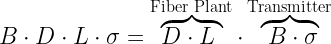
Note how each equation contains the product B∙D∙L∙σ, which I will refer to as the dispersion product. This product is the key to understanding how the G.695 specifications for dispersion were generated.

Discussion of the Dispersion Product

Equation 4 shows how we can think of the dispersion product as being composed of two terms determined by different aspects of the system: (1) a fiber plant-dependent term, and (2) a transmitter-dependent term.

Eq. 4 B\cdot D\cdot L\cdot \sigma =\overbrace{D\cdot L\text{ }}^{\text{Fiber Plant}}\cdot \overbrace{\text{ }B\cdot \sigma }^{\text{Transmitter}}

The role of the standard is to state achievable fiber plant characteristics (i.e. D·L) for which the optical manufacturers can develop interoperable optical product designs, which are can control B·σ.

Determination of the Fiber Plant Term

The specific case that I am worried about uses Corning SMF-28e fiber, which complies with ITU G.652, over an 80 km distance. This means that I can compute the fiber plant term as shown in Figure 3.

Figure 1: Computaton of the Fiber Plant Term for a 10Gbps, 80 km Fiber Link.

Figure 3: Computation of the Fiber Plant Term for a 10Gbps, 80 km Fiber Link.

ITU Assumptions for D(λ)

An industry standard has to be written so that its requirements can be met by the vast majority of manufacturers. In the case of ITU G.652, they layout their assumptions for D(λ). We can use the result of this blog post to see how the SMF-28e's D(λ) data relates to the industry standard's D(λ) assumptions (Figure 4).

Figure 3: Comparison of G.652 and SMF-28e Value for D(λ).

Figure 4: Comparison of G.652 and SMF-28e Value for D(λ).

Dispersion Power Penalty and G.695

When you look at the optics specifications for a 10 Gbps(gigbit per second) transmitter rated for 80 km, they usually assume a 1300 ps/nm dispersion "load" for test purposes. Figure 5 shows the range of power penalties we should expect to see for this optics.

Figure 4: An Example of the Dispersion Calculations.

Figure 5: An Example of the Dispersion Calculations.

These are all reasonable values for a high-end network.

Conclusion

Applying a bit of theory, I was able to reconstruct a few of the specifications from G.695 that we will be using in our work. This means that I understand what the critical parameters in the dispersion problem are and I can feel confident in moving forward -- and go to sleep.

Save

Save

Save

Save

Posted in Fiber Optics | Tagged , , | Comments Off on A Little Specification Reading Before Bed

Optical Fiber Dispersion Formula - Where Did This Come From?

Quote of the Day

I can calculate the movement of the stars, but not the madness of men.

— Isaac Newton after he lost his shirt in the South Sea Company financial bubble. He claimed to have lost over £2.4 million in today’s money. Arguably history's smartest person, even Newton could not foresee a financial meltdown.


Introduction

Figure 1: Corning Dispersion Equation from SMF-28e Specification.

Figure 1: Corning Dispersion Equation from SMF-28e Specification.

Most Fiber-To-The-Home (FTTH) deployments in North America use SMF-28e fiber from Corning, which is to fiber what Kleenex is to tissue. Unfortunately, I am so familiar with this particularly product that I can recite its specifications from memory. However, there is one aspect of SMF-28e's datasheet that I have never really understood – the chromatic dispersion formula shown in Figure 1. This formula is used to determine the fiber parameter D(λ), which specifies the travel time difference (in picoseconds [ps]) for photons that differ by 1 nm in wavelength over 1 km of fiber. Dispersion is important because an optical pulse on a fiber is made up of a range of wavelengths that will spread out as they travel down the fiber. Over a long length of fiber, this pulse spreading makes an optical signal undetectable. Dispersion sets the range limit for many fiber-based communication systems.

While looking for other fiber information, I stumbled across the rationale behind this formula and I thought I would write it down here. Let's dig in ...

Background

For general information on dispersion, the best general reference is the Wikipedia. I also have a three-part blog post on the subject.

For those who are looking for a quick description of dispersion, I will make a few points here:

  • different wavelengths of light move at slightly different speeds along a fiber.
  • digital signals are sent on a fiber in the form of pulses of optical power.
  • the pulses of optical power are generated by a laser, which produces produces optical power in a narrow range of wavelengths, usually on the order of 0.1 nm.
  • as the pulses move down the fiber, the slower wavelengths of light eventually separate from the faster wavelengths of light.
  • the separation of the wavelengths causes the pulse to spread out and eventually become impossible to detect.

Analysis

Empirical D(λ) Characteristic

Figure 2 shows D(λ) for optical fiber like SMF-28e. This figure defines two variables: (1) λ0, the zero-dispersion wavelength; (2) S0, the slope of the dispersion characteristic at λ0.

Figure 2: D(λ) Versus λ for Common Fiber Types.

Figure 2: D(λ) Versus λ for Common Fiber Types.

The Corning formula of Figure 1 uses λ0 and S0 from Figure 2 to provide us with a means of computing D(λ).

What is D(λ)?

Fiber optic systems run into problems when a significant percentage of their optical power arrives at the receiver at a different time than the rest of the optical power. We begin by deriving the transit time for light of different wavelengths over a unit length of fiber (Figure 3).

Figure 3: Definition of Transit Time Over a Unit Length of Fiber.

Figure 3: Definition of Transit Time Over a Unit Length of Fiber.

Figure 3 shows that transit time of light over a unit length of fiber is a scaled version of n(λ), the index of refraction for the glass in the fiber.

Using the argument of Figure 3, let's define the D(λ) coefficient as shown in Equation 1.

Eq. 1 \displaystyle D\left( \lambda \right)\triangleq \frac{d\left( {{\tau }_{u}} \right)}{d\lambda }=\frac{\frac{d\left( \frac{n\left( \lambda \right)}{c} \right)}{d\lambda }}{c}=\frac{\frac{dn\left( \lambda \right)}{d\lambda }}{c}

where

  • D(λ) is the dispersion coefficient at a wavelength of λ.
  • n(λ) is the index of refraction of the fiber at a wavelength of λ.
  • c is the speed of light in a vacuum.

Index of Refraction Modeling

During my investigation, I was floored at all the different approaches that have been taken for modeling the index of refraction (here is a nice summary). All of these approaches are empirical curve-fits based in some way on the Cauchy , Sellmeier , or Kettler-Helmholtz-Drude equations. Corning mentions in one of their documents that they used Sellmeier's equation. I would argue that they used a simplification of Sellmeier's equation known as Herzberger's equation, which models the index of refraction using the Laurent series shown in Equation 2.

Eq. 2 n\left( \lambda \right)=a+b\cdot {{\lambda }^{2}}+\frac{c}{{{\lambda }^{2}}}

where

  • a, b, and c are curve fitting parameters.

Derivation of the Corning Equation

We can derive Corning's dispersion formula by substituting Equation 2 into Equation 1. This equation allows us to compute D(λ) for wavelengths in the range of 1200 nm to 1625 nm using λ0 and S0 from Figure 2. The derivation is shown in Figure 4. Because I am in a bit of a hurry, I will use the Mathcad symbolic engine for the derivation, which allows me to just insert a screen capture.

Figure 4: Detailed Derivation of Corning Equation.

Figure 4: Detailed Derivation of Corning Equation.

Figure 5 shows a plot of the Corning dispersion formula.

Figure 5: Plot of the Corning Dispersion Formula.

Figure 5: Plot of the Corning Dispersion Formula.

Conclusion

This was a nice application of some elementary calculus to the derivation of a formula that optical engineers routinely use.

This derivation also allows us to physically interpret the formulas used to model dispersion. Engineers typically model the effect of dispersion using equations that are functions of \displaystyle D_0\cdot L\cdot {{\sigma }_{\lambda }} (D0= D(λ0), L= fiber length, σλ= wavelength spread of the laser). We can interpret this term as follows.

Eq. 3 \displaystyle D_0\cdot L\cdot {{\sigma }_{\lambda }}\approx \frac{\Delta {{\tau }_{u}}}{\Delta \lambda }\cdot {{\sigma }_{\lambda }}\cdot L\approx \frac{\Delta {{\tau }_{u}}}{\Delta \lambda }\cdot \Delta \lambda \cdot L=\Delta {{\tau }_{u}}\cdot L=\Delta \tau

This term represents the amount of time variation we will see in our light pulse over that length of fiber.

Save

Save

Posted in Fiber Optics | 4 Comments

Customer Service Math

While this post does not address a math problem, it does address an important aspect of mathematics -- the presentation of data. I occasionally have to prepare information on various items for our Customer Service group. For a number of years, I have maintained a graphic that shows the average cost of a kW-hr of energy by state.  Our customers use this data to estimate the yearly operating cost of our equipment in their deployments. I get the statistics from the Department of Energy (DoE) Website. It is a hassle to manually update all 50 states and DC, so I use a spreadsheet to link the data I download from the DoE to Visio. It gives me the graphic you see below. I got the original map of North America from the Visguy website.

I actually use this approach to update a number of graphics. I thought it may be useful for me to include it here as a model for people to use when linking Excel data to Visio. I have included a link at the bottom of this post to a zip file that contains the Excel spreadsheet and Visio drawing I use. When you extract the files, they will go into a directory called "North America." Just run the Visio file from that directory. It should be able to find the spreadsheet. I do not know how to setup a relative address in Windows, but this works on my machines.

You can force an update of the graphic by going to the Visio data tab and clicking refresh all.

Here is my source material: NorthAmerica.zip

Save

Posted in Management | 12 Comments

Phone Loads For Backup Time Testing

Introduction

I often have to assist with writing test procedures. One of our procedures involves testing the battery backup time for the equipment we install at the subscriber's home, which is called an Optical Network Unit (ONU). Nearly all ONUs installed in the United States are installed with an Uninterruptible Power Supply (UPS) because phone service in the US is considered a safety-critical service, which means it must work during a power failure. Oddly enough, almost no ONUs installed internationally use a UPS and they simply use a "wall wart" for their power conversion.

The math in this post will be simple, but it is the sort of thing I end up doing all the time. Our customers need procedures that they can use to compute things like:

  • battery backup time
  • battery lifetime
  • yearly power cost to subscribers (the homeowners pay for the ONU's power)

In all these cases, I use weighted averages to simplify calculations or procedures. In the particular case that I am going to explain here, I will be using a weighted average to simplify a routine test procedure.

Background

Telecommunications service requirements in the US are still strongly influenced by the legacy of the Bell System. In the case of battery backup time, telecom companies expect their ONUs to have 8 hours of backup time when tested according to specifications from Telcordia, the company that now controls the old Bell System specifications. We use Telcordia specification GR-909 for backup time tests, which states (with some editing):

The system supplier shall specify the battery reserve time, multiplied by 0.8, obtained under the following conditions:

The ONU primary power source shall be removed. One-half of the equipped single-party message telephone lines shall be off-hook. After three hours, only one-sixth of the single-party message telephone service lines shall remain off-hook. The remaining lines shall be on-hook.

If you think it sounds complicated now, you should have seen it before I removed all the boiler plate.

Our customers expect a minimum of 8 hours of ONU backup time when tested according to this procedure. I interpret the procedure above to mean that I need to guarantee 10 hours of backup time with a new battery at this level of phone loading in order to claim 8 hours of backup time (10.0 hours · 0.8 = 8.0 hours). While this sounds odd, it is consistent because GR-909's requires the replacement of any battery that has aged to less than 80% of it rated capacity. So GR-909 wants to ensure 8 hours of backup time even with an old battery. It also means that I always test with new batteries.

While we run this exact test procedure for final acceptance testing, we use a simplified procedure for routine prototype testing. We have seen that our simplified procedure always provides the same result as the specified procedure and it is simpler to execute in practice.

Simplified Procedure Derivation

Phones only put a significant load on a system when they are off-hook. It is a hassle for engineers to constantly put combinations of phones off-hook and on-hook at specific times. For prototype testing (i.e. not final acceptance tests), the easiest way for the testers to work is to put a specified number of phones off-hook for a specified amount of time and then put the phone back on-hook when that time is over.

To generate an equivalent load, I begin by computing the total phone load (phone · time) experienced by an ONU during testing. I then create a equivalent load profile that does not require the testers to worry about the details of phone ratios and times.

Figure 1 shows how I computed that effective number of off-hook phones for a ten hour period.

Figure 1: Computation of Effective Phone Load.

Figure 1: Computation of Effective Phone Load.

Since we cannot have a fractional phone but can have a fractional hour, we can compute how long to keep a number of phones off-hook in order to have the same loading as specified by GR-909 (see Figure 2).

Fiigure 2: Number of Phones and their Off-Hook Times to Duplicate GR-909 Requirements.

Figure 2: Number of Phones and their Off-Hook Times to Duplicate GR-909 Requirements.

All this means that we can get a GR-909 equivalent load by using the following procedure:

  • For a 2 phone ONU → one phone off-hook for 5 hours and 20 minutes during the ten hour test.
  • For a 4 phone ONU → two phones off-hook for 5 hours and 20 minutes during the ten hour test.
  • For a 8 phone ONU → three phones off-hook for 7 hours and 6 minutes during the ten hour test.

Conclusion

This post illustrates how you can use a weighted average to compute the equivalent load of a more complicated test procedure. While it does not replace the more complicated procedure, it does provide a simple way to easily test prototypes prior to the final acceptance test.

Posted in Electronics | Comments Off on Phone Loads For Backup Time Testing

Dimensional Analysis and Submarine Running Time

Introduction

Part of my job is looking at backup power sources for remote telecommunications gear. I recently have been doing some reading on fuel cells, which we are starting to see in some backup power applications. I started googling to see if I could find other fuel-cell applications and I found a paper on fuel cell usage in modern diesel electric submarines. This paper contained the following graph (Figure 1).

Figure 1: German HDW Type 214: Submerged Propulsion Performance

Figure 1: German HDW Type 214: Submerged Propulsion Performance

Figure 1 shows this submarine's submerged running time at a given speed for battery-only (blue line) and battery plus fuel cell power (red line). I am going to focus on the battery-only power curve in my discussion here.

In an earlier post, I reviewed a video by John Barrow on the dimensional analysis of Olympic rowers. I am going to expand that discussion and show how it applies to Figure 1 and submarines. It turns out that rowers and submarines have a lot in common.

Problem Description

Submerged underwater vehicles are powered by energy sources that do not require air. Excluding nuclear power, which is only an option for the military of a major power, batteries have been the most commonly used energy source. Unfortunately, batteries have a low energy density and they tend to be big and heavy (i.e. most submarine batteries use lead-acid chemistry).  Because underwater propulsion is all about energy, the key Figure of Merit for an underwater propulsion system is its total available energy.

While energy is the critical parameter in underwater propulsion, it is frequently seen in a hidden form. For example, consider the table shown in Figure 2, which is from a US Navy historical web site. It contains a common nautical FOM, R·v2.

Figure 2: US Navy Table on Torpedo Performance.

Figure 2: US Navy Table on Torpedo Performance.

This FOM is really just a way to state the propulsion energy present in the system. Figure 3 illustrates how to derive this relationship.

Figure 3: Derivation Showing Propulsion FOM is a Restatement of Energy.

Figure 3: Derivation Showing Propulsion FOM is a Restatement of Energy.

The analysis of Figure 3 tells us the energy expended to move through the water, but it does not represent the total energy expended because it does not include any inefficiencies in the system associated with generating that motion. In the case of rowers, to put a given amount of energy into moving a boat through the water you must actually start with more energy because there will be losses. For example, some additional energy is required to keep the rower's bodies functioning and to generate waves. In a submarine, some energy must be expended for life support and operating its control systems (e.g. navigation, steering, sensors). The following analysis will assume that the drag force on a submarine is proportional to its velocity squared and that the submarine has a constant power load that adds to its propulsion power usage.

Analysis

My analysis process is simple:

  • Model the submarine power usage as a combination of propulsion and non-propulsion loads
  • Capture submarine performance data in Figure 1 so that I can analyze it.
  • Plot the actual submarine performance against the load model to see how it compares.

I was pleased with how well this model was able to match the empirical data of Figure 1.

Model of Submarine Propulsion and Non-Propulsion Load

Since Figure 1 shows submarine speed versus time, we need to develop a relationship between submarine energy and speed. The US Navy FOM discussed above relates speed to range. However, range = speed · time, so we can develop another relationship as shown in Figure 4 below.

Figure 4: Energy is Proportional to Time Multiplied by Speed Cubed.

Figure 4: Energy is Proportional to Time Multiplied by Speed Cubed.

We can now augment this model with a constant non-propulsion power load (called the "hotel load"). The derivation in Figure 5 illustrates my modeling approach.

Figure 5: Derivation of Speed Versus Time Model Equation.

Figure 5: Derivation of Speed Versus Time Model Equation.

Submarine Speed Versus Run Time Curve Capture

I captured the data from the online pdf using Dagra and put that data into Mathcad. Figure 6 shows the result.

Figure 6: Captured Submarine Data.

Figure 6: Captured Submarine Data.

Combined Loss Model and Comparison with Reality

In Figure 7, I have a comparison of my fitted model with the actual submarine performance curve. If I assume that PHotel/k = 83, I get an almost exact fit.

Figure 7: Comparison of Actual Submarine Performance to Model Prediction.

Figure 7: Comparison of Actual Submarine Performance to Model Prediction.

In Figure 7, we see how ignoring the hotel load gives a reasonably close approximation, but including the hotel load makes the model prediction almost identical to the empirical data.

Conclusion

While a bit complicated, this post shows that the analysis used to model the performance of an Olympic row boat applies to a submarine if losses are included.

Posted in Electronics | 3 Comments

Battery Self-Discharge Math

Quote of the Day

Life isn't about finding yourself. Life is about creating yourself.

— George Bernard Shaw:"


Introduction

7.2 A-hr Sealed Lead Acid Battery.

Figure 1: 7.2 A-hr Sealed Lead Acid Battery.

I deal with a lot of battery issues. Our products generally ship with an Uninterruptible Power Supply (UPS) that contains a 7.2 A-hr Sealed Lead-Acid (SLA) battery (Figure 1). I occasionally hear customers say that we shipped them bad batteries. Since we charge the batteries just before shipment, I know the batteries left our facility functional and with a full charge. In every single case, the customer had not properly handled the batteries -- the batteries had become fully discharged because they had been stored for too long between charging cycles. A discharged lead-acid battery will eventually become sulfated -- a state where the battery plates are coated with a crystalline layer of lead sulfate and lead oxide. Some people refer to this layer as a "varnish" because sulfated plates look like they are coated with wood varnish. A sulfated battery usually is only good for recycling. See the Appendix of this post for a reference on the topic.

During a normal discharge cycle, lead-acid batteries form a layer of amorphous lead sulfate on their plates. Charging converts the amorphous form of lead sulfate back to lead. Unfortunately, when a discharged battery is stored for a long period of time (usually weeks or months), the amorphous lead sulfate changes into a crystalline form that cannot be converted back to lead through normal charging. This paper has great photos that actually show you the crystals that form.

When I first started this job, I would often go to the deployment sites to investigate reports of customers receiving dead batteries. My first customer visit was pretty typical. The customer was angry that all of his batteries were dead. I started my investigation by asking him how he handled his batteries. He told me that his UPS units were stored in warehouse prior to being installed. I asked him if I could visit the warehouse and he proceeded to take me to a large barn. The UPS units and their batteries were stored in the loft of the barn at a temperature of about 50°C (122 °F). They typically sat in the warehouse for three to four months before being deployed. The batteries were dying during that storage period. I told my customer that the batteries were not being stored according to the vendor's battery storage requirements. He said that no one ever told him what the battery handling requirements were and I needed to pay to replace every one of his failing batteries (including service call). I then reached into a UPS box and pulled out the battery handling specification that ships with every UPS. He seemed pretty sheepish after seeing that he had received thousands of battery handling instruction sheets. He had never actually looked in the boxes.

At room temperature, batteries can sit for months without a problem. However, batteries at high temperature can fail in a very short period of time. Let's examine this acceleration closer.

Background

Few batteries die a natural death -- most batteries are murdered. They are murdered by owners that charge them improperly, cycle them too deeply, let them sit discharged for too long, or store them at too high a temperature. Since our UPS units have built-in controllers and the units are rarely deeply discharged, the primary battery killer is heat.

Batteries are electrochemical machines. Chemical reactions govern how they work and chemical reactions govern how they fail. Chemical reactions exist within a battery that cause them to discharge while just sitting in storage. Other chemical reactions cause them to form crystalline lead sulfate. Both of these reactions are accelerated by temperature according to the Arrhenius equation, which I state in Equation 1.

Eq. 1 k=A \cdot {{e}^{-{{E}_{a}}/R \cdot T}}

where

Equation 1 tells us that increasing temperature produces an exponential increase in reaction rate. Let's examine how this reaction rate affects a battery that appears to just be sitting there -- it actually is experiencing an internal chemical reaction that is discharging the battery. I also want to examine a common rule of thumb for electrical engineers.

A battery at a temperature of T+10 °C self-discharges twice as fast as the same battery at a temperature of T.

Is this rule true? If it is true, the customer that I mentioned earlier who stored his batteries at 50 °C would see his batteries discharged in his warehouse within about two and half months. At that point, the sulphation process begins. His batteries were dying right before his eyes.

Analysis

Empirical Battery Discharge Data

All battery vendors publish self-discharge data for their products. Each battery vendor's products have different self-discharge rates because the rates are a function of how the plates are constructed (i.e. different lead alloys). Figure 2 shows a particularly well done self-discharge chart.

Figure 1: Sealed Lead Acid Battery Self-Discharge Graph.

Figure 2: Sealed Lead Acid Battery Self-Discharge Graph.

Discussion

I am not an electrochemist and I will not discuss all the details of Equation 1, but we can learn some things from a qualitative examination of Figure 1.

  • A lead-acid battery self-discharges over time.
  • The chart shows that you do not want to let a battery discharge below 60% of its full capacity.
  • A lead-acid battery can be stored for about a year at room temperature before it needs a recharge.
  • At high temperature (i.e. >40°C), a battery self-discharges much more rapidly than at room temperature (~22 °C).

It is amazing how many batteries I have seen destroyed by high temperature. At one deployment site, I saw that the customer had over 900 batteries reported as failures. Every failed battery had been stored improperly and then installed in a private residence when fiber service was installed at that home. The UPS did a battery load test every ten days, so the battery would be reported as failed 10 days after it was installed, which means a technician had to physically go out to a person's home and replace the failed battery (often with another failed battery). This went on for a year.

I would not want to explain to my boss that I screwed up by not following the directions included with every battery. Replacing a battery is not cheap, and paying for a service call to install the battery is not cheap either. There were many tens thousands of dollars worth of avoidable problems at this one customer site alone.

Rule of Thumb Accuracy

Assume that we want to ensure that our batteries never drop below 60% of full charge. In Figure 1, we see that as the battery temperature raises from 30 °C to 40 °C, the self-discharge time reduces from 8 months to about 5 months, which is less than half. We also see that as the battery temperature raises from 25 °C to 40 °C, the self-discharge time reduces from 13 months to about 5 months, which is more than half. So the actual doubling (or halving) temperature difference is between 10 °C and 15 °C. So the rule of thumb appears to provide a pessimistic answer in this case, which is okay for a rule of thumb.

Note that the exponential function and the rule of thumb are only related approximately. The derivation in Figure 3 shows that the rule of thumb is only true for a limited range of values. However, the range of values is reasonable with respect to lead-acid batteries.

Figure 2: Derivation Showing Approximate Equivalence of Rule of Thumb and Arrhenius Equation.

Figure 3: Derivation Showing Approximate Equivalence of Rule of Thumb and Arrhenius Equation.

Appendix Reference

The derivation shows that the 1/10.25 K is the proportionality "constant" for temperatures near 22 °C (room temperature) --the slow variation of the logarithm function helps us here. This means that the reaction rate roughly doubles for a 10.25 °C increase in temperature. The "constant" varies a bit across the temperature range of a battery. Figure 4 shows this variation. For a rule of thumb, it is not bad.

Figure 3: Variation in C parameter of Alternate Arrhenius Function.

Figure 4: Variation in C parameter of Alternate Arrhenius Function.

Conclusion

As summer nears, I will again receive calls from people about dead batteries. I hope I can provide guidance to people on how to avoid a costly and avoidable error.

Appendix

Activation Energy

Figure 5 is an excerpt from a battery reference ("Valve-Regulated Lead-Acid Batteries" by David Anthony and James Rand) that provides a value for the activation energy for the self-discharge reaction in a lead-acid battery.

Figure 4: Activation Energy Reference.

Figure 5: Activation Energy Reference.

Discussion of the Crystalline Layer

Figure 6 is an excerpt from page 16 of "Valve-Regulated Lead-Acid Batteries" by David Anthony and James Rand that discusses the formation of an insulating layer.

Figure 5: Reference on Forming an Insulating Layer That Renders Batteries Unchargeable.

Figure 6: Reference on Forming an Insulating Layer That Renders Batteries Unchargeable.

Save

Save

Posted in Electronics | Tagged , | 8 Comments