Quote of the Day
A satisfied customer is the best business strategy of all.
— Michael LeBoeuf, writer and management professor.
Introduction

Figure 1: Multiple antenna elements makes beamforming possible. (Source)
I was at the Consumer Electronics Show (CES) last week and spent a lot of time talking to various silicon vendors about their wireless offerings. During these discussions, the topic of beamforming came up numerous times. Beamforming maximizes the transmit energy and receive sensitivity of an antenna in a specific direction. Beamforming is becoming a critical technology for improving the data transfer rate of wireless systems -- rates that are critical to making wireless technology a credible option for delivering reliable Internet Protocol (IP) video around a home. The reliable delivery of IP video over wireless will simplify the deployment of Fiber-to-the-Home systems (my focus) by eliminating the need to install Ethernet cables to every room, which is expensive.
These discussions brought back many memories. Years ago, I spent a lot of time working on beamforming for military sonar and radar systems. Military and aerospace technology often finds a home in commercial applications once it becomes cost effective, and beamforming is now becoming inexpensive enough to be in every home. Because I was familiar with the technology, I decided that it would be worthwhile to put together some training material for my staff on how beamforming works. I began by writing a Mathcad worksheet for simulating a simple linear antenna array. This simulation seemed to be a good way to illustrate how beamforming works and I thought it would be worthwhile to cover here.
Background
Let's begin by defining beamforming. As usual, let's turn to the Wikipedia.
Beamforming is a signal processing technique used in sensor arrays for directional signal transmission or reception. This is achieved by combining elements in the array in a way where signals at particular angles experience constructive interference and while others experience destructive interference. Beamforming can be used at both the transmitting and receiving ends in order to achieve spatial selectivity. The improvement compared with an omnidirectional reception/transmission is known as the receive/transmit gain (or loss).
I really like this definition because it focuses on the critical role of interference in allowing us to either direct energy (acoustic or electromagnetic) in a desired direction or to receive energy from a desired direction. Using advanced methods, we can also reject sending or receiving energy from a specific direction, which is called null steering. Beamforming will be my focus here.
Beamforming is useful for wireless communication because these systems have limited transmit power and it is best to point the energy you transmit toward an actual receiver. When you are receiving, it is best to listen carefully in the direction of a transmitter and to reject noise coming from other directions. Null steering is useful when you have source of interference that you wish to reject, which could be something as common as a microwave oven making popcorn or a neighbor's wireless system.
Since beamforming is a such a good thing to do, let's now take a closer look at how it works.
Analysis
All mathematics going forward are done using complex numbers.
Reciprocity
As mentioned above, beamforming can be applied to both transmitting and receiving. In fact, transmit and receive beamforming are identical because of the principle of reciprocity, which states that the receive sensitivity of an antenna as a function of direction is the same as the transmit radiation pattern from the same antenna when transmitting. See the Wikipedia for a discussion of this topic.
Linear Antenna Array
For the purposes of this post, I will use the simple model of a linear array shown in Figure 1.
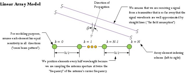
Figure 1: Linear Antenna Model.
To keep this discussion simple, I will make the following assumptions:
- The antenna is composed of a series of identical elements separated by λ/2, where λ= c/f, c is the speed of light, and f is the frequency of transmission.
Since the dawn of radio, engineers have been directing radio power along specific directions using shaped reflectors (e.g. parabolas). You can analyze antenna arrays using the viewpoint that we are sampling these apertures using small antennas that I will refer to here as elements. Since we are sampling an aperture, λ/2 makes sense because it corresponds to the Nyquist sampling rate for a receiver with a wavelength of λ. I will not be taking a sampling viewpoint for the remainder of this post, but I may in future posts.
- Every element is a receiver -- I will ignore transmitting.
By the reciprocity theorem, everything I say for a receiving antenna will also be true for a transmitting antenna. I am making this assumption just to reduce the amount of redundancy in this discussion. You should think of every element as a small antenna. We are going to be working with arrays of small antennas.
- The receiver elements generate an output voltage or current that is proportional to the level of the signal impinging upon it.
This means that that output of an antenna element is an accurate reproduction of the signal strength impinging upon it.
- Every element has an omnidirectional sensitivity response.
This means that every element is equally sensitive in all directions.
- Assume that the wavelength λ = 1.
Expressing all lengths in units of λ does not limit this discussion in any way and is simpler to deal with analytically. This means that the elements are separated by 1/2 in units of λ.
Given these assumptions, we can now create a mathematical model for the receive output of a linear array as a function of beam angle. While the linear array example is simple to analyze, it does illustrate the basic approach to analyzing larger and more complex antenna arrays.
Simple Beamforming Algorithm
What is Beamforming Computationally?
Beamforming computationally is simply the linear combination of the outputs of the elements, which a beam can be computed using Equation 1.
| Eq. 1 |
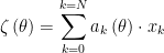 |
where
- N is number of elements.
- k is an index variable.
- ak is the complex coefficient of the kth element.
- xk is the voltage response from the kth element.
- ζ is the beam response.
- θ is the angle of the beam main lobe.
Equation 1 is not difficult to compute, but we need to determine what coefficients we should use to enhance the antenna's receive gain in a specified direction. The mathematics behind computing these coefficients is covered below.
Intuitive View of Array Beamforming
Consider Figure 2, where we have a transmitter that is far away from our linear antenna. "Far away" in this case means that the transmitter is many wavelengths distant from the receiving antenna.

Figure 2: Illustration of the Phase Shift At Each Element.
For a transmitter that is far enough away, the wavefronts can be approximated as plane waves when they arrive at the receive antenna. When we evaluate Equation 1 for the situation shown in Figure 2 assuming that ak=1 , the maximum response is generated when all wavefronts hit each element at the same time (perfect constructive interference). This will occur when the transmitter is located on a line that is perpendicular to the orientation of the linear array. If the transmitter moves away from the perpendicular, destructive interference begins to occur and the magnitude of the response reduces.
In order to steer the beam in different directions, we need to look closely at Figure 2 and observe that, for transmitters that are not along the perpendicular, there is a linearly increasing phase shift introduced along the array elements. Can we use the coefficients to cancel out the phase differences and rotate the direction of maximum antenna response? It turns out we can.
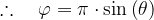
We can compute the phase shift in the signal received between each element using Equation 2. The key to deriving this equation is to note that each element receives the same signal, but at a slightly different time. This time delay can be modeled as a phase shift in the frequency domain.
where
- θ is the angle of target relative to a vector normal to the center of the element array.
- φ is the phase shift between each element.
- δt is the time delay of the signal between the elements.
- f is the transmit frequency.
- c is the speed of light.
- t is time.
If we can compensate for the phase shift, we can maximize our receiver's response in the direction of the transmitter. That is exactly what we are going to do.
Beamforming Simulation
Here is the approach I am going to use to determine the output of a simple beamformer.
- Determine the distance from each element to the source using the Pythagorean theorem.
- Determine the amplitude and phase of the signal at each element using the distance.
- Evaluate Equation 1.
- Plot the output of Equation 1 as a function of transmitter angle.
Distance to the Transmitter
Equation 3 shows my Mathcad program for generating the distance between an element and the transmitter.
| Eq. 3 |
 |
where
- N is number of elements.
- r is the radial distance to the transmitter.
- θ is the angle of target relative to a vector normal to the center of the element array.
- k is the element index (labeled from left to right in Figure 1).
Amplitude and Phase of the Received Signal
Equation 4 gives the phase of the signal at element as a function of distance. This formula uses the fact that each wavelength of distance equals 2·π of phase.
| Eq. 4 |
 |
Evaluate Equation 1
My approach to evaluating Equation 1 is to break it into three parts.
- Generate a vector of steering coefficients.
- Compute a matrix of the element responses over a range of transmitter angles.
- Form the matrix product of the steering coefficients and the element responses, which is equivalent to evaluating Equation 1.
Figure 3 illustrates how I compute the compensating phase shifts for two different beams. It turns out that you can generate multiple beams in parallel and I will illustrate below.

Figure 3: Generate the Coefficients For Generating a Beam in A Specific Direction.
Figure 4 illustrates how to compute a matrix of element responses for a transmitter positioned along a range of angles from 0° to 180°.

Figure 4: Element Responses for a Range of Angles from 0° to 180°.
Plot the Output of Equation 1
Figure 5 shows a plot of sensitivity for two beams, at 45° and -30° off the perpendicular (b1 contains the coefficients for 45° and b2 contains the coefficients for -30°).

Figure 5: Two Beam Patterns for a 7 Element Antenna and a Transmitter at Range = 1000 λ.
Conclusion
There is a lot more to talk about here, but I was able to put together a simple beamforming example for my team. You can see from this example that one can "point" the response curve of the antenna in specific direction with just a bit of matrix math. Note that the antenna beam patterns have a main "lobe" and side "lobes." In a later post, I will discuss how to reduce the amplitude of the sidelobes.
Save
Save


 .
.
 , which is true in this case. Equation 2 shows how to compute the Normal approximation to the Poisson calculation of Figure 1.
 . Thus,
  .
.


![d{{B}_{Approx}}(x)=\left[ {{a}_{4}}\quad {{a}_{3}}\quad {{a}_{2}}\quad {{a}_{1}}\quad {{a}_{0}} \right]\cdot {{\left[ {{x}^{4}}\quad {{x}^{3}}\quad {{x}^{2}}\quad x\quad 1 \right]}^{T}}](https://s0.wp.com/latex.php?latex=d%7B%7BB%7D_%7BApprox%7D%7D%28x%29%3D%5Cleft%5B+%7B%7Ba%7D_%7B4%7D%7D%5Cquad+%7B%7Ba%7D_%7B3%7D%7D%5Cquad+%7B%7Ba%7D_%7B2%7D%7D%5Cquad+%7B%7Ba%7D_%7B1%7D%7D%5Cquad+%7B%7Ba%7D_%7B0%7D%7D+%5Cright%5D%5Ccdot+%7B%7B%5Cleft%5B+%7B%7Bx%7D%5E%7B4%7D%7D%5Cquad+%7B%7Bx%7D%5E%7B3%7D%7D%5Cquad+%7B%7Bx%7D%5E%7B2%7D%7D%5Cquad+x%5Cquad+1+%5Cright%5D%7D%5E%7BT%7D%7D&bg=ffffff&fg=000&s=1&c=20201002)