Quote of the Day
If Hitler invaded hell, I would have had a nice word or two for the devil in the House of Commons.
— Sir Winston Churchill, his response when asked why he was saying nice things about the Soviet Union after Hitler invaded the Soviet Union.
Introduction

Figure 1: Typical Thermistor Construction and Symbols (Source).
A common electrical engineering task during the design of a circuit card is designing a way for the circuit to measure its own temperature. Knowing the temperature of a circuit board is important for compensating for component temperature variations and diagnosing heat problems. Normally, I use a thermistor as my temperature probe. A thermistor is a resistor whose resistance varies with temperature (Figure 1). The thermistors that I use have a negative temperature coefficient (NTC), which means their resistance reduces as their temperature increases. In many ways, thermistors are a great sensor: cheap, tough, small, and accurate.
Thermistors have one major drawback – their resistance variation with temperature is non-linear. Figure 2 shows how the resistance of a typical NTC thermistor varies with temperature.

Figure 2: Resistance Versus Temperature for a Murata NCP03XM102 05RL Thermistor.
Linearity is a sensor characteristic that is loved by analog engineers. For this kind of problem, it means that calibration is simple (i.e. two points determine a line) and I do not need a processor around to implement complex compensation equations. The resistance characteristic of an NTC thermistor is too non-linear for my application directly. But what if I combined the NTC thermistor with other components in a manner that would somehow tame this non-linear response? This post will look at a common approach to linearizing the circuit response from a thermistor.
Problem Description
All engineering problems begin with determining requirements. Here is how I see my requirements for this problem:
- Limited range of temperatures to be measured
I only need to measure temperature over a limited temperature range (0 °C to 40 °C). This is considered the standard temperature range for indoor applications.
- Minimal calibration
Sensors usually require calibration, which is an expensive operation in production.
- Generates a voltage that varies linearly (approximately) with temperature.
I want a linear sensor to simplify my calibration. A linear sensor requires a couple of measurements to complete calibration.
- Temperature accurate within 5 °C.
This level of accuracy means that I can get by with an approximately linear sensor.
- Minimal impact on software
My processor is a very limited microprocessor (i.e. AVR) with minimal memory. I will use an analog-to-digital converter in the processor to read the voltage. I want the conversion from voltage to temperature to very simple. I have neither the memory nor time to require any fancy curve interpolation to get a simple temperature reading.
- Minimal Printed Circuit Board (PCB) space because I only have space for a couple 0603-sized (i.e. 0.6 mm x 0.3 mm) components. Instead, you could consider contacting a PCB software specialist company for advice or help with this electrical engineering task (such as Altium for example).
- Minimal cost
I need something that costs pennies.
- No integrated circuits.
I am not wild about using an IC in this application. There are quite a few ICs that put out a voltage that is Proportional to Absolute Temperature (PTAT), but they generally require a power supply voltage that I do not have available or they cost too much.
Thermistor Characteristics
The resistance characteristic of Figure 1 can be modeled in a number of ways, but only two are really seen often: the Steinhart-Hart equation, and the ß-Parameter Equation.
The classic approach is the Steinhart-Hart equation (Equation 1). It is a very accurate model. In fact, it is far more accurate than I need.
| Eq. 1 |
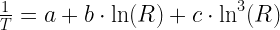 |
where
- a, b, c are parameters that are chosen to fit the equation to the resistance characteristic.
- R is the thermistor resistance (Ω).
- T is the thermistor temperature (K)
While the Steinhart-Hart equation may be accurate, I have found it useless for use by an analog designer in a hardware application. It is simply too difficult to work mathematically without substantial software resources.
The ß-Parameter Equation is much more interesting to an analog engineer. Equation 2 shows the ß-Parameter Model as it is usually seen.
| Eq. 2 |
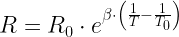 |
where
- R0 is the themistor resistance at temperature T0
- ß is a curve fitting parameter.
The ß-Parameter Model is sufficiently accurate for my purposes and is much simpler to work with mathematically than the Steinhart-Hart equation. We will use this model for the remainder of this post.
Thermistor Linearization
Approach
Most thermistor linearization approaches involves adding parallel or series resistors. I will use a thermistor with a series resistor configured as a voltage divider (see Figure 3). This is the simplest linearization circuit that I can think of.

Figure 3: Simple Series Resistor Circuit for Thermistor Linearization.
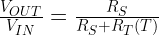
We will be measuring the output voltage (VOut) from the voltage divider, which is given by Equation 3.
| Eq. 3 |
 |
where
- VIN is the voltage divider drive voltage.
- VOUT is the voltage divider output voltage.
- RS is the resistance of the series resistance.
- RT(T) is the resistance of the thermistor.
To get an intuitive feel for the how the linearization occurs, you need to consider the asymptotic cases. For low temperatures, RT(T) is large relative to RS and the output is approximately  , which approaches 0 as the temperature drops. For high temperatures, RT(T) is small relative to RS and the output voltage approaches VIN. Figure 4 shows the thermistor resistance and the normalized output voltage versus temperature.

Figure 4: Example of a Thermistor's Resistance and the Linearized Voltage Divider Ratio.
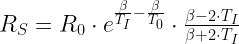
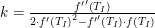
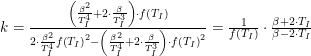
Look closely at Figure 4 and you will see an inflection point in the curve (452 Ω and 50 °C in Figure 4). At the inflection point,  . After a long, tedious derivation (shown in the Appendix below), one can show that the inflection point can be moved where you want it by changing RS. Equation 4 shows the relationship between the temperature of the inflection point and the value of RS.
| Eq. 4 |
 |
where
- TI is the temperature of inflection.
- T0, R0 ,and ß are thermistor parameters given by the thermistor vendor.
The "rule of thumb" is to select RS to place the inflection point in the middle of your temperature range of operation. As you can see in Figure 4, this placement helps to minimize the maximum deviation from a line through the inflection point. However, it is not guaranteed to be the point of minimum error. When I need that level of accuracy, I use numerical methods to find the RS that minimizes the maximum error.
Example
Figure 5 shows a worked example of my thermistor calculations in Mathcad.

Figure 5: Example of Thermistor Calculations for Series Linearization.
Conclusion
The design of the linearization circuit for a thermistor is a nice use of basic calculus in an engineering application. Hopefully, some of you will find all the details presented useful.
Appendix
I wanted to record my derivation of Equation 4 so I would not have to go through the derivation pain again later, but since it is long and tedious I did not want to put readers through it – an Appendix seemed the appropriate place.
My approach is straightforward:
- Develop an expression for VOUT using the ß-Parameter model.
- Take the first and second derivatives of this expression.
- Set the second derivative equal to zero.
- Solve this expression for RS.
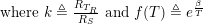
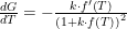
The derivation is shown in Equation 5. I will let the details stand for themselves.
You can also derive Equation 4 using Mathcad, which I demonstrate in Figure 6. The main issue with my Mathcad derivation is that many of the details are hidden. However, it took me less than a minute to complete it.

Figure 6: Mathcad Derivation of Equation 4.
Save
Save
Save


 .
.