Speed of a Meteor

Quote of the Day

Failure is an option here. If things are not failing, you are not innovating enough.

— Elon Musk


Introduction

Figure 1: Meteor at Twilight.

Figure 1: Meteor at Twilight. (Source)

One of my coworkers knows one of my brothers (I have three). My brother and this coworker are friends and their families vacation together. They happened to be at a lake one night in Northern Minnesota together and my brother showed this coworker where to look for satellites and meteors. This coworker stopped by my desk and told me about the great time they had just watching the sky and how interesting it was.

I own a small cabin on a lake in Northern Minnesota. Years ago I showed my brother how to find satellites, planets, and meteors. I love to lay on the dock at night and watch the sky. Because Northern Minnesota is so sparsely populated, the sky is incredibly dark and the stars are so much brighter than in the metropolitan region where I spend most of my time. When people visit me at the cabin, I take them out on the dock and introduce them to the world of meteors, satellites, and planets. It is always a good time.

During a recent discussion on our sky-watching activities, a coworker mentioned that some meteor showers have "fast" meteors and some have "slow" meteors. Why are some meteors fast and others slow? What does fast mean? What does slow mean? This is another example of a Fermi problem and some simple mathematics will give us a feel for what the answer is.

Background

Meteor Shower Basics

I am not an expert on meteors, so I needed to do some research. It turns out there are three sources of meteors:

  • Asteroid belt
    The asteroid belt is the source of the slow-moving meteors, which are assumed to originate from collision between objects in the asteroid belt. The Geminides are a good example of this type of meteor shower.
  • Comets
    Comets have often been compared to "dirty snowballs" that orbit the Sun. They release rocky material as the heat of the Sun causes them to slowly disintegrate. Comets are the source of the fast-moving meteors. The Leonids are a good example of this type of meteor shower.
  • Outside of the Solar System
    These are very rare and unpredictable, so they would not be part of any well-known meteor shower. However, their velocity could be very high as they would not be in orbit of the Sun (by definition) and would be following hyperbolic trajectories. I will not be addressing this case here. However, one case has been discovered and it was moving very fast.

Computing Escape Velocity

All estimates of meteor velocity that I have seen involve a discussion of escape velocity. Escape velocity is the lowest velocity that a body must have in order to escape the gravitational attraction of a particular planet or other object.

We can compute the escape velocity by computing the work that a massive body does on a meteor. Equation 1 gives us the force on the meteor exerted by the gravity of an attracting body.

Eq. 1 {{F}_{Meteor}}=G\cdot \frac{{{M}_{Body}}\cdot {{m}_{Meteor}}}{{{r}^{2}}}

where

We can use Equation 1 to derive Equation 2, which is the work (i.e. energy) performed on the meteor by the gravitational field of the attracting body.

Eq. 2 {{E}_{Meteor}}=\int\limits_{\infty }^{{{R}_{Body}}}{-{{F}_{Meteor}}\left( r \right)}\cdot dr=G\cdot \frac{{{M}_{Body}}\cdot {{m}_{Meteor}}}{{{R}_{Body}}}

where

  • EMeteor is the work performed on the meteor by the attracting body.
  • RBody is the radius of the attracting body (I am assuming the attracting body is spherical).

Equation 3 equates the kinetic energy of the meteor with the work performed on the meteor by the attracting body.

Eq. 3 \frac{1}{2}\cdot {{m}_{Meteor}}\cdot v_{Meteor}^{2}=G\cdot \frac{{{M}_{Body}}\cdot {{m}_{Meteor}}}{{{R}_{Body}}}\Rightarrow {{v}_{Meteor}}=\sqrt{2\cdot \frac{G\cdot {{M}_{Body}}}{{{R}_{Body}}}}

where vMeteor is the speed of the meteor. We will use Equation 3 to estimate the speed of the meteors entering our atmosphere.

Analysis

Asteroid-Based Meteor Shower

In this case, we assume that the meteor has somehow broken free of an asteroid with negligible velocity and has simply fallen to the Earth. This means that its velocity at the surface of the Earth will be the escape velocity from the Earth. Figure 2 illustrates the calculation.

Figure 2: Illustration of Velocity for a Meteor Originating in the Asteroid Belt.

Figure 2: Illustration of Velocity for a Meteor Originating in the Asteroid Belt.

This calculation explains the 11 km/s speed sometimes quoted for slow meteors.

Comet-Based Meteor Shower

Comets orbit the Sun and the meteors generated by comets move at the velocity of a comet. These meteors really are orbiting the Sun and just happen to slam into the Earth. Figure 3 illustrates the calculation of their velocity.

Figure 3: Velocity of a Meteor Originating from a Comet.

Figure 3: Velocity of a Meteor Originating from a Comet.

This calculation explains the 42 km/s mentioned in the Wikipedia. The Wikipedia also mentions the peak velocity is 71 km/s, which is the speed of a comet-based meteor slamming heading on into an Earth that is moving at 29 km/s around the Sun.

Conclusion

I have seen the speed of meteors estimated to be anywhere from 11 km/s to 71 km/s. This post has shown where these numbers come from and they appear to be reasonable.

Save

Posted in Astronomy | 28 Comments

How to Interview Engineers

Quote of the Day

If something is important enough you should try, even if the probable outcome is failure.

- Elon Musk


Introduction

Figure 1: Team Interviewing.

Figure 1: Team Interviewing. (Source)

My youngest son has a long drive to and from work everyday. During his drive home, he frequently calls me to help him pass the time. During a recent drive, we talked about how I interview engineers, which I have done hundreds of times. I have a fairly standard interview methodology. The key part of any interview is how you go about grading the applicants.

In a previous post, I mentioned that I look for three things:

  • Pisstivity
  • Anality
  • Prima Donna Factor

My son was wondering what questions do I ask, and if they were anything like the challenging microsoft interview questions. Clearly, it was different from what he thought, and I explained it to him. He seemed to think the discussion was interesting and I thought it was worthwhile capturing some of it here.

Interview Process

I should go through my interview process quickly. From my point of view, there are three parts:

  • resume review
  • phone screen
  • in-person interview

I depend on the resume and phone screen to tell me if the candidate has the technical chops to work in my group. The resume gives me a feel for the candidates general work history. It also shows me how well they present information. An engineer must be able to write to work in my group. During the phone screen, I ask a lot of questions about things like their projects, the roles they played, and tools they have used (e.g. simulation, schematic capture, etc).

During the in-person interview, I really am looking at how well the person interacts with people. My basic approach is to start off with a few minutes of chit-chat to try to put the candidate at ease. After that, I try to find out what drives the person. I focus on questions like:

  • What project gave you the most satisfaction during your career?
  • Tell me about a project where you really made a difference technically?
  • What me about a project where you really made a difference non-technically (e.g. organizer, facilitator, mentor)?
  • Do you do anything technically in your spare time (e.g. astronomy, amateur radio, car stuff)

When I mentioned my questions, my son said that he has seen a good list of questions in a paper by a person named Buckingham that were similar to mine. Here are Buckingham's questions:

  1. What was the best day at work you've had in the last three months?
  2. What was the worst day at work you've had in the last three months?
  3. What was the best relationship with a manager you've ever had?
  4. What was the best praise or recognition you've ever received?
  5. When in your career do you think you were learning most?

Questions 1 and 2 give you an idea of the candidate's work values. Questions 3 and 4 tell you how a manager can motivate them. Question 5 tells you about their learning style.

Conclusion

I like Buckingham's questions and I have incorporated them into my basic set of interview questions. I am always looking for good interview questions. If any readers have questions they like to ask, please drop me a comment and tell me what you ask.

Posted in Management | 1 Comment

Another Analog Design Legend Dies

Quote of the Day

Politics is ethics done in public.

— Bernard Crick


Figure 1: Bob Pease, Analog Legend.Figure 1: Bob Pease, Analog Legend.

Figure 1: Bob Pease, Analog Legend. (Source)

I just saw the announcement that Bob Pease died in a car accident after leaving a memorial to Jim Williams, another analog legend. This is very sad. I have read everything that Bob Pease wrote. His column for Electronic Design, "Pease Porridge," was required reading for my crowd.

Jim Williams and Bob Pease were very important to the current generation of analog designers. They will be missed.

Posted in Electronics | Comments Off on Another Analog Design Legend Dies

Density of a Neutron Star

Quote of the Day

Some people get rich studying artificial intelligence. Me, I make money studying natural stupidity.

— Carl Icahn


Introduction

Figure 1: Example of Neutron Star System.

Figure 1: Example of Neutron Star System. (Source)

Television science programs frequently talk about black holes and neutron stars. A common quote during these programs is something like "a teaspoon of neutron star stuff weighs a billion tons" or some other similar statement. I always find numbers like these interesting to look at in detail.

Let's dig in  ...


Background

We are going to estimate the average density of a neutron stars, which means that we need to get some mass and volume information.

  • According to the Chandrasekhar limit, a neutron star must have a mass at least 1.44 times that of the Sun (mass of the Sun = 1 solar mass).
  • According to the Tolman-Oppenheimer-Volkoff limit, the upper limit on a neutron star's mass is between 2 and 3 solar masses. Collapsing stars more massive than the TOV limit form black holes instead of neutron stars.
  • The radius of a neutron star is between 10 and 15 km

My calculation is for the average density of neutron star stuff. Note that a neutron star does have structure and it is composed of material whose properties vary with distance from the core.

During my research, it became very clear that the physics of matter in neutron stars and black holes is still being worked out. As in every field, to really know a subject you must understand the corner cases and astronomers are still working this area out. Personally, I think its great because this means that there is more interesting science to come.

Analysis

Figure 2 shows the details of my analysis.

Figure 1: Estimate of Neutron Star Density.

Figure 2: Estimate of Neutron Star Density.

So my estimate is ~2 billion tons for a teaspoon of neutron star stuff. Since this is a Fermi-type problem, my estimate agrees with the statement of one billion tons per teaspoon.

How does the average density of a neutron star compare to the density of neutron? Figure 3 shows my estimate for the density of a neutron.

Figure 2: Estimate of a Neutron's Density.

Figure 3: Estimate of a Neutron's Density.

So the average density of a neutron and a neutron star are pretty much the same.

Conclusion

A neutron star does have a density of about a billion tons per teaspoon. Pretty incredible number when you think of it.

Save

Save

Save

Posted in Astronomy | Comments Off on Density of a Neutron Star

The Papoulis Filter (aka Optimum "L" Filter)

Quote of the Day

Two things prevent us from happiness; living in the past and observing others.

— Pinterest


Introduction

Figure 1: Athanasios Papoulis. (Source)

Figure 1: Athanasios Papoulis. (Source)

Analog engineers often have to design filters, which generally entails a lot of polynomial manipulation. Since I am currently designing some active filters, I thought it would be worthwhile documenting a filter function that I am using right now, but that is not widely known. This is the Papoulis or Optimum "L" filter. For this article, I will refer to this filter as the "L-filter." The "L" stands for Legendre, a mathematician whose like named polynomials are used in the derivation of the function.

This particular post made extensive use of Mathcad's symbolic processor. I left pretty impressed with what it could do.


Background

Most active filters are designed using one of four filter functions:

  • Butterworth
    This is a very friendly filter function. It has the flattest of all passbands and tends to have a well-behaved transient response because its poles are relatively low Q. Unfortunately, its roll-off rate is rather poor.
  • Chebyshev
    This filter is covered in every filter textbook, but I have actually never been able to use it. I have never been able to tolerate the ripple it creates in the passband. It does have very good roll-off characteristics.
  • Bessel
    I use this one a lot. The Bessel filter's linear phase characteristic gives it the best behaved transient response of all the filter functions, but its roll-off rate is very poor.
  • Cauer (Elliptic)
    I have used the Cauer filter quite a bit. It allows ripple in the stopband, which I usually can tolerate. It is a bit complicated to design and it has high-Q poles, which can create transient response problems.

These four filters have always been more popular than the L-filter. However, I certainly have had more use for the L-filter than for the Chebyshev. Since I was going through a design, I thought I would document it here.

History

The L-filter was developed by Athanasios Papoulis in a pair of articles published in 1958 and 1959:

  • odd-ordered polynomial: "Optimum Filters with Monotonic Response," Proc. IRE, 46, No. 3, March 1958, pp. 606-609
  • even-ordered polynomial:"On Monotonic Response Filters," Proc. IRE, 47, No. 2, Feb. 1959, 332-333 (correspondence section)

For a given filter order, the L-filter has the fastest roll-off rate of all filters with a monotonic magnitude response (i.e. the low-pass filter magnitude function always decreases with increasing frequency). I have used this filter a number of times in situations where I needed a relatively flat filter response and a sharp roll-off.

Comparison with Other Filter Functions

Figure 2 shows how the L-filter compares to the Butterworth and Chebyshev filters (all 3rd order in the figure).

Figure 1:Comparison of L-Filter, Butterworth, and Chebyshev Magnitude Characteristics.

Figure 2:Comparison of L-Filter, Butterworth, and Chebyshev Magnitude Characteristics.

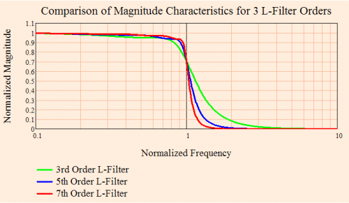
Figure 3 shows how the L-filter characteristics change as the L-filter order increases.

Figure 2: Comparison of L-Filter Magnitude Characteristics for 3rd, 5th, and 7th Orders.

Figure 3: Comparison of L-Filter Magnitude Characteristics for 3rd, 5th, and 7th Orders.

Analysis

Function Definition

The definition of the L-filter function is rather complicated. Because I am mathematically lazy, I will be using Mathcad's symbolic processor to perform all the manipulations.

Legendre Polynomials

For detailed information on the Legendre polynomials, the Wikipedia is about as good as it gets. I chose to generate the polynomials using the recurrence relation shown in Equation 1.

Eq. 1 {{P}_{i}}\left( x \right)=1\quad i=0
{{P}_{i}}\left( x \right)=x\quad i=1
{{P}_{i}}\left( x \right)=\frac{\left( 2\cdot i-1 \right)\cdot x\cdot {{P}_{i-1}}\left( x \right)-\left( i-1 \right)\cdot {{P}_{i-2}}\left( x \right)}{i}\quad \text{otherwise}

n Odd

Equation 2 generates L(ω²) for filters of odd order.

Eq. 2 {{L}_{n}}\left( \omega _{n}^{2} \right)={{\int\limits_{-1}^{2\cdot {{\omega }_{n}}-1}{\left( \sum\limits_{i=0}^{k}{{{a}_{i}}\cdot {{P}_{i}}\left( x \right)} \right)}}^{2}}dx

where

  • Pi are the Legendre polynomials of the first kind.
  • ωn is the normalized frequency variable \left( {{\omega }_{n}}\triangleq \frac{\omega }{{{\omega }_{3\text{dB}}}},\text{ where }{{\omega }_{3\text{dB}}}=2\cdot \pi \cdot {{f}_{3\text{dB}}} \right)
  • f3dB is the 3 dB bandwidth of the filter.
  • \omega \triangleq 2\cdot \pi \cdot f,\text{ where }f\text{ is frequency}\text{.}
  • {{a}_{i}}\triangleq \frac{2\cdot i+1}{\sqrt{2}\cdot \left( k+1 \right)},\text{ where }k=\frac{n-1}{2}

n Even

Equation 3 generates L(ω²) for filters of even order.

Eq. 3 {{L}_{n}}\left( \omega _{n}^{2} \right)={{\int\limits_{-1}^{2\cdot {{\omega }_{n}}-1}{\left( x+1 \right)\cdot \left( \sum\limits_{i=0}^{k}{{{a}_{i}}\cdot {{P}_{i}}\left( x \right)} \right)}}^{2}}dx

where {{a}_{i}}\triangleq \frac{2\cdot i+1}{\sqrt{\left( k+1 \right)\cdot (k+2)}}, i\text{ even, 0 otherwise }\left( k=\frac{n-2}{2} \right).

Mathcad Routine for Determination of the L(ω²) function

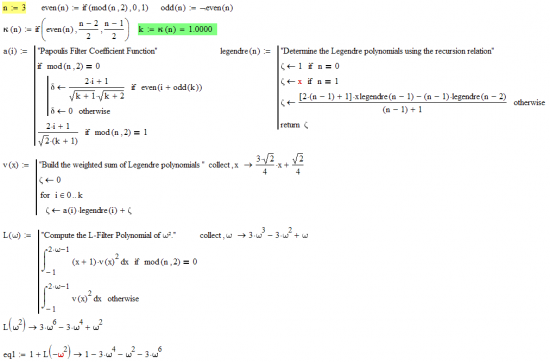
Figure 4 shows the Mathcad routine that I developed to generate the Ln(ω²)(Equation 3).

Figure 3: Mathcad Routine for Determination of the L-Function.

Figure 4: Mathcad Routine for Determination of the L-Function.

Mathcad Routine for Determination of Filter Function

Figure 5 shows the Mathcad routine that I used to generate the actual filter function and my graphs.

Figure 4: Mathcad Routine for Generation of the Filter Function.

Figure 5: Mathcad Routine for Generation of the Filter Function.

L(ω2) Function

Table 1 shows the L(ω²) polynomials. Some folks have documented these polynomials instead of the characteristic polynomials. These polynomials are not directly useful for designs, but some web sites list them and they are useful for comparison purposes (i.e. verifying that my algorithm implementation is working correctly).

Table 1: L(ω²) Polynomials.
n L\left( {{\omega }^{2}} \right)
1 {{\omega }^{2}}
2 {{\omega }^{4}}
3 3\cdot {{\omega }^{6}}-3\cdot {{\omega }^{4}}+{{\omega }^{2}}
4 6\cdot {{\omega }^{8}}-8\cdot {{\omega }^{6}}+3\cdot {{\omega }^{4}}
5 20\cdot {{\omega }^{10}}-40\cdot {{\omega }^{8}}+28\cdot {{\omega }^{6}}-8\cdot {{\omega }^{4}}+{{\omega }^{2}}
6 50\cdot {{\omega }^{12}}-120\cdot {{\omega }^{10}}+105\cdot {{\omega }^{8}}-40\cdot {{\omega }^{6}}+6\cdot {{\omega }^{4}}
7 175\cdot {{\omega }^{14}}-525\cdot {{\omega }^{12}}+615\cdot {{\omega }^{10}}-355\cdot {{\omega }^{8}}+105\cdot {{\omega }^{6}}-15\cdot {{\omega }^{4}}+{{\omega }^{2}}
8 490\cdot {{\omega }^{16}}-1680\cdot {{\omega }^{14}}+2310\cdot {{\omega }^{12}}-1624\cdot {{\omega }^{10}}+615\cdot {{\omega }^{8}}-120\cdot {{\omega }^{6}}+10\cdot {{\omega }^{4}}
9 1764\cdot {{\omega }^{18}}-7056\cdot {{\omega }^{16}}+11704\cdot {{\omega }^{14}}-10416\cdot {{\omega }^{12}}+5376\cdot {{\omega }^{10}}-1624\cdot {{\omega }^{8}}+276\cdot {{\omega }^{6}}-24\cdot {{\omega }^{2}}+\cdot {{\omega }^{2}}
10 5292\cdot {{\omega }^{20}}-23520\cdot {{\omega }^{18}}+44100\cdot {{\omega }^{16}}-45360\cdot {{\omega }^{14}}+27860\cdot {{\omega }^{12}}-10416\cdot {{\omega }^{10}}+2310\cdot {{\omega }^{8}}-280\cdot {{\omega }^{6}}+15\cdot {{\omega }^{4}}

Filter Characteristic Function (s domain)

Table 2 shows the optimum L characteristic polynomials for n = 1 to 10.

Table 2: Optimum L Characteristic Polynomials.
n D\left( s \right)
1 \text{s+1}\text{.0}
2 {{s}^{2}}+1.4142 \cdot s+1
3 {{s}^{3}}+1.3107\cdot {{s}^{2}}+1.359039\cdot s+0.57736522
4 {{s}^{4}}+1.5628\cdot {{s}^{3}}+1.8878811\cdot {{s}^{2}}+1.2414681\cdot s+0.40821577
5 {{s}^{5}}+1.5515\cdot {{s}^{4}}+2.2034703\cdot {{s}^{3}}+1.692534\cdot {{s}^{2}}+0.89817083\cdot s+0.22356064
6 {{s}^{6}}+1.7262\cdot {{s}^{5}}+2.6898696\cdot {{s}^{4}}+2.4335933\cdot {{s}^{3}}+1.6332102\cdot {{s}^{2}}+0.67969552\cdot s+0.14143644
7 {{s}^{7}}+1.72772\cdot {{s}^{6}}+2.9926117\cdot {{s}^{5}}+2.9244072\cdot {{s}^{4}}+2.3320509\cdot {{s}^{3}}+1.2307095\cdot {{s}^{2}}+0.43791348\cdot s+0.075589885
8 {{s}^{8}}+1.86148\cdot {{s}^{7}}+3.4468776\cdot {{s}^{6}}+3.7236172\cdot {{s}^{5}}+3.3481719\cdot {{s}^{4}}+2.1192882\cdot {{s}^{3}}+0.99411199\cdot {{s}^{2}}+0.29972527\cdot s+0.045184527
9 {{s}^{9}}+1.8665\cdot {{s}^{8}}+3.7418201\cdot {{s}^{7}}+4.249464\cdot {{s}^{6}}+4.2481258\cdot {{s}^{5}}+3.0122773\cdot {{s}^{4}}+1.7075194\cdot {{s}^{3}}+0.68048233\cdot {{s}^{2}}+0.1815741
10 {{s}^{10}}+1.9744\cdot {{s}^{9}}+4.1713498\cdot {{s}^{8}}+5.0886545\cdot {{s}^{7}}+5.5135609\cdot {{s}^{6}}+4.3545176\cdot {{s}^{5}}+2.8312648\cdot {{s}^{4}}+1.3753686\cdot {{s}^{3}}+0.49627083\cdot {{s}^{2}}+0.11679607\cdot s+0.013743239

Factored D(s) for Single and Double Pole Realizations

When I design active filters, I usually implement them as quadratic and simple pole sections. This means the factored form of the denominator polynomial is easier for me to design with. Table 3 shows the factored form of the polynomials from Table 2.

Table 3: Factored Optimum-L Filter Polynomials.
n Factored D(s)
1 \text{s+1}\text{.0}
2 {{s}^{2}}+1.4142 \cdot s+1
3 \left( \text{s+0}\text{.6203} \right)\cdot \left( {{s}^{2}}+0.6904\cdot s+0.9308 \right)
4 \left( {{s}^{2}}+1.0994\cdot s+0.4308 \right)\cdot \left( {{s}^{2}}+0.4634\cdot s+0.9477 \right)
5 \left( \text{s+0}\text{.4681} \right)\cdot \left( {{s}^{2}}+0.7762\cdot s+0.4971 \right)\cdot \left( {{s}^{2}}+0.3072\cdot s+0.9608 \right)
6 \left( {{s}^{2}}+0.6180\cdot s+0.5830 \right)\cdot \left( {{s}^{2}}+0.8778\cdot s+0.2502 \right)\cdot \left( {{s}^{2}}+0.2304\cdot s+0.9696 \right)
7 \left( \text{s+0}\text{.3821} \right)\cdot \left( {{s}^{2}}+0.6984\cdot s+0.3060 \right)\cdot \left( {{s}^{2}}+0.4748\cdot s+0.6621 \right)\cdot \left( {{s}^{2}}+0.1724\cdot s+0.9765 \right)
8 \left( {{s}^{2}}+0.6006\cdot s+0.3829 \right)\cdot \left( {{s}^{2}}+0.3886\cdot s+0.7180 \right)\cdot \left( {{s}^{2}}+0.13788\cdot s+0.9809 \right)\cdot \left( {{s}^{2}}+0.7344\cdot s+0.1676 \right)
9 \left( \text{s+0}\text{.3257} \right)\left( {{s}^{2}}+0.3146\cdot s+0.7666 \right)\cdot \left( {{s}^{2}}+0.6188\cdot s+0.2090 \right)\cdot \left( {{s}^{2}}+0.4972\cdot s+0.4635 \right)\cdot \left( {{s}^{2}}+0.1102\cdot s+0.9845 \right)
10 \left( {{s}^{2}}+0.5548\cdot s+0.2702 \right)\left( {{s}^{2}}+0.0918\cdot s+0.9870 \right)\cdot \left( {{s}^{2}}+0.4284\cdot s+0.5282 \right)\cdot \left( {{s}^{2}}+0.2650\cdot s+0.8013 \right)\cdot \left( {{s}^{2}}+0.6344\cdot s+0.1218 \right)

Conclusion

My hope is that this post will help folks who find the need for another filter function option. I have found this function useful in a number of cases and maybe you will too.

Save

Save

Posted in Electronics | 13 Comments

The Passing of an Analog Electronics Giant

Quote of the Day

The difference between successful people and very successful people is that very successful people say 'no' to almost everything.

— Warren Buffet


Figure 1: Jim Williams, Analog Legend.

Figure 1: Jim Williams, Analog Legend. (Source)

I just saw the announcement that Jim Williams passed away. This guy was an inspiration to me. His apps work at National Semiconductor was a model for the industry. His articles in magazines like EDN provided real-world examples of elegant analog design techniques. His books, particularly Analog Circuit Design: Art, Science and Personalities, provided wonderful examples of problem solving. He will be missed.

I always smiled when I read his bio -- he had majored in psychology and did not have an engineering degree. I have worked with a number of self-taught engineers (Javi Sanchez is another). These folks are forces of nature. They are driven to design circuits.

One other thing -- photos of his desk always showed it to be messier than mine. That somehow always made me feel better about the clutter that I seem unable to avoid.

Posted in Electronics | Comments Off on The Passing of an Analog Electronics Giant

Filter Design Details

Quote of the Day

Torture the date, and it will confess to anything.

— Ronald Coase, data scientist


Introduction

Figure 1: Examples of Filter Rolloffs.

Figure 1: Examples of Filter Roll Offs. (Source)

During a recent circuit design review, I saw the need for a simple two-pole filter in one region of the circuit. As I thought about, this filter might be a good example to work through here in the blog. While the application is rather routine, it does illustrate the general process involved in designing one of the most common forms of a low-pass filter.

This is also good application for a computer algebra system. I chose Mathcad, which did a very nice job.

Requirements

I am constantly amazed at how many people try to "short-change" the amount of effort they spend on determining requirements. I make sure that I have the requirements fully determined before I start designing. As far as I am concerned, every minute spent working on the wrong problem is a minute wasted.

This does not mean that determining requirements is easy. I refer to this process as "The Treasure Hunt." Requirements are my treasure and, like any real treasure, you may have to look hard to find it. In this case, the requirements were pretty obvious:

  • The output of the filter is a quasi-DC voltage level (i.e. it changes slowly and infrequently)
    We are using the PWM generator followed by this filter to build a "poor man's" a digital-to-analog converter (DAC). We are working with a very low-cost device that has a PWM generator but not a DAC. Our cost goals are so tough that we cannot afford to add a DAC.
  • The input to the filter is a pulse train that is pulse-width modulated.
    As mentioned above, we have a PWM generator available for free and we want to re-task it for use as a DAC.
  • The input level is from 0 to 1 V with a modulation rate of 100 kHz.
    The PWM generator uses 100 kHz switching frequency and we need to filter this component out to achieve a smooth enough DC level.
  • The output level is from 0 to 5 V and is to be a DC level with less than 0.5 mV of ripple.
    We need a relative steady voltage level. With an input amplitude of 1 V and an output amplitude of 5 V, it also means we need a circuit with some gain.
  • The circuit is not sensitive to offset voltage or any of the other op-amp imperfections.
    Some applications are very sensitive to common-mode errors, offset voltage, or bias currents. This application in not one of those.

Design

Approach

Given the operational requirements listed above, we can derive some design requirements as shown below.

  • I need to attenuate the PWM-induced voltage ripple by at least 4 orders of magnitude (5 V/10,000 = 0.5 mV).
  • Attenuation by a factor of 10,000 means 80 dB of attenuation \left( 20\cdot \log \left( \text{10,000} \right)=80\text{ dB} \right).
  • As a working assumption, set fBW = 100 Hz.
    This means we will have 3 decades of frequency rolloff to reduce the filter gain down by 80 dB or more. A wider transition region reduces the order of the filter required.
  • A 2-pole filter should provide more than enough attenuation.
    A 2-pole filter provides 40 dB of attenuation per decade of frequency rolloff. A 2-pole filter should be able to meet 80 dB of attenuation over 2 decades of frequency rolloff. Since we have 3 decades of frequency rolloff to work with (100 Hz to the 100 KHz PWM frequency), I should actually see 120 dB of attenuation (more is good). So I will set the filter bandwidth at f_{BW} = \text{100 Hz}.
  • The circuit needs a gain of 5 at DC (0 Hz)
    Basically, the circuit will need to amplify a pulse train with a 1 V peak amplitude to a DC level with a 5 V peak amplitude.
  • The circuit needs to have a low output impedance.
    This means that I really would like to have the voltage come directly off of the output of an opamp.

The circuit does not have stringent transient response requirements. I just need a nice, stable, filter circuit (i.e. no high Q poles). In this situation, many engineers will choose a Sallen-Key circuit configured to implement a Butterworth filter. That is exactly what I will do here.

Butterworth Polynomial

Implementing a Butterworth filter means coming up with a physical realization of a Butterworth polynomial. Normally, I just read the polynomial from a table. For illustrative reasons, I will forgo the table look-up and will derive the second-order Butterworth polynomial using the key defining characteristic of a Butterworth polynomial – maximal flatness at 0 Hz.This same approach can be used to determine the Butterworth polynomial of any order. I will also show any other Butterworth polynomial can be found.

Maximal flatness means that the first n-1 derivatives of the magnitude-squared function {{\left| G(j\cdot \omega ) \right|}^{2}} equal 0 at 0 Hz. Most filter design work (analog and digital) is done using the magnitude-squared function {{\left| G\left( j\cdot \omega \right) \right|}^{2}}. This is because {{\left| G\left( j\cdot \omega \right) \right|}^{2}} can always be expressed as a real-function of ω2\left( {{\left| G\left( j\cdot \omega \right) \right|}^{2}}=f\left( {{\omega }^{2}} \right) \right). As you will see below, this makes taking derivatives fairly simple.

We can set the first n-1 derivatives to zero because (1) we have n coefficients (i.e. n degrees of freedom), and (2) we use one degree of freedom when we set {{\left| G(j\cdot {{\omega }_{BW}}) \right|}^{2}}=\frac{1}{2}. With a second-order filter, this means that the first derivative of {{\left. \frac{d}{d{{\omega }^{2}}}{{\left| G\left( j\cdot \omega \right) \right|}^{2}} \right|}_{\omega =0}}=0.

Equation 1 shows the general 2-pole, low-pass, magnitude-squared function.

Eq. 1 {{\left| G\left( j\cdot {{\omega }_{n}} \right) \right|}^{2}}=\frac{{{K}^{2}}}{1+A\cdot {{\omega }_{n}}^{2}+B\cdot {{\left( {{\omega }_{n}}^{2} \right)}^{2}}}

where

  • K is the gain at 0 Hz (5 in this case).
  • A, and B are polynomial coefficients.
  • {{\omega }_{n}}\triangleq \frac{\omega }{{{\omega }_{3\text{dB}}}}

In Figure 2, I use Mathcad's symbolic solver to show that A = 0 and B = 1.

Figure 1: Derivation of the Magnitude Squared Function.

Figure 2: Derivation of the Magnitude Squared Function.

In Figure 1, we derived the magnitude squared function {{\left| G\left( j\cdot \omega \right) \right|}^{2}}=\frac{25}{1+{{\left( {{\omega }^{2}} \right)}^{2}}}=\frac{25}{1+{{\omega }^{4}}}. We can use the magnitude squared function to derive the Butterworth filter function (Figure 3).

Figure 2: Derivation of the Second-Order Butterworth Polynomial.

Figure 3: Derivation of the Second-Order Butterworth Polynomial.

Thus, the second order Butterworth polynomial is s_{n}^{2}+\sqrt{2}\cdot {{s}_{n}}+1, where sn is the normalized Laplace frequency variable. This polynomial agrees with that listed for the second-order in this table of Butterworth polynomials.

We can prove that the general form of the magnitude-squared form of a Butterworth Polynomial of order n is 1-{{\left( \omega _{n}^{2} \right)}^{2}}. Figure 4 shows how Mathcad can be used to generate a table of Butterworth polynomials.

Figure 3: Mathcad Program for Generating a Table of Butterworth Polynomials.

Figure 4: Mathcad Program for Generating a Table of Butterworth Polynomials.

Sallen-Key Circuit

Figure 5 shows the Sallen-Key circuit, which is a very commonly used circuit for this type of application.

Figure 4: Sallen-Key Low-Pass Filter Circuit.

Figure 5: Sallen-Key Low-Pass Filter Circuit.

I have used this circuit many times with much success.

Analysis of Sallen-Key Circuit

Figure 6 shows a standard Kirchoff's Voltage Law (KVL) analysis of the Sallen-Key circuit.

Standard Solution

Figure 5: Equations for the Sallen-Key Circuit.

Figure 6: Equations for the Sallen-Key Circuit.

I usually do not work with filter equations in the form shown in Figure 5. I like to normalize the frequency variable, s, relative to the filter bandwidth ({{s}_{n}}\triangleq \frac{s}{2\cdot \pi \cdot {{f}_{BW}}}).

Normalized Form

Figure 7 shows the Butterworth equation normalized to the filter bandwidth. This is the equation form normally shown in the filter design tables.

Figure 6: Development of the Normalized Form of the Butterworth Filter.

Figure 7: Development of the Normalized Form of the Butterworth Filter.

Component Determination

Figure 8 shows how we can determine the component values required for this implementation using the equation solving abilities of Mathcad.

Figure 7: Determination of the Passive Components Value.

Figure 8: Determination of the Passive Components Value.

We can now generate a plot of the filter magnitude characteristic using these component values.

Gain Characteristic

Figure 9 shows the gain characteristic of this design. As expected, we are seeing 120 dB of ripple attenuation. The gain at 0 Hz is 5, so that requirement is also met.

Figure 8: 2-Pole Butterworth Gain Characteristic.

Figure 9: 2-Pole Butterworth Gain Characteristic.

Conclusion

This was a good example of a common filter design problem. I have used both circuit simulators and computer algebra software to design these filters. I have come to like computer algebra software for this kind of work because it gives me equations. These equations allow me to see how the output varies as a function of individual component values. This means that I can see useful approximations.

Save

Posted in Electronics | 3 Comments

Solar Photons

Quote of the Day

Forgiveness is the final form of love.

— Reinhold Niebuhr


Introduction

Figure 1: Our Sun. (Source)

Figure 1: Our Sun. (Source)

I was watching "How the Universe Works" on the Science Channel and they had a really interesting discussion on stars and photons. During the show, they mentioned that photons generated in the center of the Sun take 4000 years to get to the surface. From the surface, the photons only take 8 minutes to get to the Earth. As part of my campaign to promote active television watching, let's take a look at where these numbers come from. As part of this effort, I will use Mathcad for the calculations and as a programming tool for a simple simulation.


8 Minutes to Earth

This is an easy one and Figure 2 illustrates the calculation. In this calculation, dAU is the distance from the Sun to the Earth, and c is the speed of light.

Figure 1: Confirmation of 8 Minute Transit Time.

Figure 2: Confirmation of 8 Minute Transit Time.

4000 years to the Surface

I had to think about this one a bit. I want to treat this like a Fermi problem (i.e. an exercise in rough approximation). Basically, a photon in the center of the Sun has to play a game of pinball with all the atoms in there on its way to the Surface. The classic way to model this situation is as a random walk. Let's look at how we can model a random walk process.

Random Walk Modeling

For simplicity, let's assume that we can model the photon as traveling an average distance l between each interaction with an atom. When a photon interacts with an atom, it is re-emitted in a random direction. I will ignore any time associated with the re-emission. Since it is a photon, it travels at a velocity c between the interactions. The mean distance, \overline{d}, that a random walker travels from its point of origin is given by Equation 1.

Eq. 1 \overline{d}=l\cdot \sqrt{N}

where

  • l is the length between interactions.
  • N is the number of interactions.
  • \overline{d} is the mean distance traveled.

We can derive this expression for the one-dimensional case as shown in Equation 2. For this case, the random iterates all have equal magnitudes, but random signs.

Eq. 2 d={{l}_{1}}+{{l}_{2}}+\cdots +{{l}_{N}}
\left\langle {{\overline{d}}^{2}} \right\rangle =\left\langle {{\left( {{l}_{1}}+{{l}_{2}}+\cdots +{{l}_{N}} \right)}^{2}} \right\rangle
{{\overline{d}}^{2}}=\left\langle {{l}_{1}}\cdot {{l}_{1}}+{{l}_{2}}\cdot {{l}_{2}}+\cdots +{{l}_{N}}\cdot {{l}_{N}}+{{l}_{1}}\cdot {{l}_{2}}+{{l}_{1}}\cdot {{l}_{3}}+\cdots +{{l}_{N-1}}\cdot {{l}_{N}} \right\rangle
{{\overline{d}}^{2}}=\sum\limits_{i=1}^{N}{\underbrace{\left\langle {{l}_{i}}\cdot {{l}_{i}} \right\rangle }_{={{l}^{2}}}}+2\cdot \underbrace{\sum\limits_{i\ne j}{\left\langle {{l}_{i}}\cdot {{l}_{j}} \right\rangle }}_{=0}=N\cdot {{l}^{2}}
{{\overline{d}}^{2}}=N\cdot {{l}^{2}}
\therefore \overline{d}=l\cdot \sqrt{N}

We can illustrate how this equation works with a simple simulation.

Equation Verification Through Simulation

Figure 3 shows a Mathcad program for simulating a two-dimensional random walk of 5000 steps (variable N) 100 times (variable n). I will not go into detail here, but the results for 1, 2, and 3 dimensional random walks are the same.

Figure 2: Mathcad Simulation of a Two-Dimensional Random Walk.

Figure 3: Mathcad Simulation of a Two-Dimensional Random Walk.

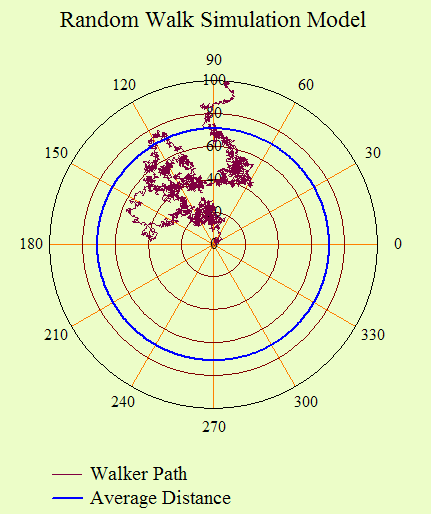
The simulation uses complex numbers to make the path vector easily rotatable. I have set the interaction distance l to 1 for the demonstration. Figure 4 shows the result of one of trials from the program in Figure 3.

Figure 3: Simulation Results from a Single Trial.

Figure 4: Simulation Results from a Single Trial.

For 500 trials of 5000 interactions, the simulation computed a mean random walk distance of 69.4, while theory predicts 70.7 (Equation 1). The agreement is pretty good.

Solar Transit Time Calculation

We can compute an estimate for a photon's solar transit time as shown in Figure 5, which shows a simple pair of equations being solved simultaneously. In this system, I first solve for the number of interactions N. The transit time \tau can then be computed by assuming the photon traveled a distance of N \cdot l at a speed of c. For our rough analysis, we will assume that the average free path, l, for a photon is ~1 cm. Determining this number is complicated and I will refer you to this reference.

Figure 4: Calculation of the Transit Time for A Photon Through the Sun.

Figure 5: Calculation of the Transit Time for A Photon Through the Sun.

My result is ~5000 years, which is close to the 4000 years stated in the program.

Conclusion

I was able to derive the results stated in the program and got a feel for some of the dynamics going on inside of the Sun. All of the numbers associated with the Sun are so large that they always leave me in awe.

Save

Posted in Astronomy, General Science | 2 Comments

Chili Math and a Good Use for Decibels

Quote of the Day

It takes as much energy to wish as to plan.

— Eleanor Roosevelt


Introduction

You never know what you will see when you walk into a guy's cube. I went to an engineer's cube with a simple question on some electronic parts and I left with an education on chili peppers. My education began when I looked at his bookshelf and noticed that it was filled with various hot sauces, a dead giveaway that I was in the presence of a man who likes his heat. I also noticed the following chart on one of his walls (Figure 1).

Figure 1: Scoville Chile Heat Mask.

Figure 1: Scoville Chile Heat Mask.

Some of you may be familiar with the Scoville scale, but I was not. As far as culinary heat is concerned, I break into a sweat just walking near a Jalapeno pepper.

The Wikipedia has good discussion of the Scoville scale and its history, so I will not go into that here. My interest is in the dynamic range of the Scoville scale. Pure capsaicin, the heat-producing component in chile, has a Scoville rating of 15,000,000. A Belle pepper has a Scoville rating of near 0.

It is rare to see this kind of dynamic range in everyday life. It is here that I see a good use for decibels ...

Convenient Numbers

For those of you who are not familiar with the decibel (abbreviated dB), it is computed as shown in Equation 1.

Eq. 1 dB(x)=10\cdot \log \left( x \right)

I use decibels everyday, but I have never really liked them. Much of my dislike has to do with how they are used. I see people treat decibels as a unit, but they really are not a unit – decibels are a scaling. I see two main reasons to use decibels.

  • To compress physical measurements into a more friendly-number range.
    Human beings can only visualize a limited range of numbers. Because of our decimal orientation, engineers frequently try to use scalings that put frequently used numbers in the range of 0 to 100. The decibel does compress an amazing number of physical quantities into the range of 0 to 100.
  • The decibel converts multiplication into addition.
    This is the most important feature of the decibel and why engineer's specify so many system parameters in decibels. Because many systems have transfer functions that involve products of numbers, the use of decibels allows one to compute complex values using simple addition.

So while I see uses for the decibel, some guys take it to a ridiculous level. I know of at least one engineer who can figure out interest rates, car payments, and all sorts of compound interest calculations in his head by using dBs. It may be hard to believe, but even I think that is obsessive.

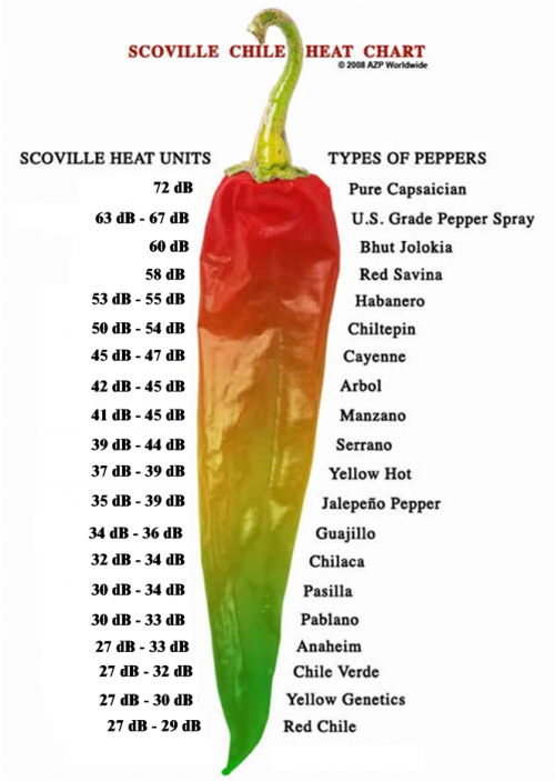
Anyway, I think that the Scoville range of 0 to 15,000,000 is way too big for a human to visualize. I think that dB could help here. Figure 2 shows Figure 1 expressed in dB. I think these numbers are easier to work with.

Figure 2: Scoville Scale in dB. I like these numbers better

Figure 2: Scoville Scale in dB. I like these numbers better

Posted in Baking, General Mathematics | 3 Comments

The Power of a Simple Magnifying Glass

Introduction

My favorite radio program is Science Friday. Last week, their web page included an excellent video where Science Friday's resourceful intern, Flora Lichtman, gave a wonderful explanation behind the use of a lens to concentrate the Sun's power. Her assistant in this effort was Thomas Baer, Executive Director of the Stanford Photonics Research Center (i.e. big shot). Here is a link to the video.

http://www.sciencefriday.com/embed/video/10380.swf

During the demonstration, they did bit of math that showed how a person could compute the level of solar power concentration provided by a simple magnifying glass. In a manner totally appropriate for this kind of video, they magically pulled out an equation and a value for the angular diameter of the Sun (Flora did say to look up the angular diameter of the Sun in any physics textbook). I thought it would be worthwhile to derive both the equation and the angular diameter of the Sun. Let's dig in ...

Analysis

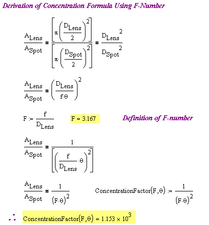
During the video, Thomas Baer wanted to give a simple, approximate formula for the concentration factor of solar power provided by a common magnifying glass. He gave the formula shown in Equation 1.

Eq. 1 \text{Concentration Factor}={{\left( \frac{100}{F} \right)}^{2}}

where F is the F-number of the lens. The F-number of the lens is defined as F=\frac{f}{D_{Lens}}, where f is the focal length and DLens is the diameter of the lens. For the lens in their example, they computed an F-number of about 3.16, which means the concentration factor is 1000. This means that the power at the spot is the same as what entered the lens, but it is concentrated on an area 1000 times smaller.

I want to derive Equation 1 from first principles. We can start with Figure 1, which illustrates the geometry of the situation.

Figure 1: Illustration of the Magnifying Glass Scenario.

Figure 1: Illustration of the Magnifying Glass Scenario.

Determination of the Angular Diameter of the Sun

Figure 2 illustrates how to calculate the Sun's angular diameter at the Earth (Ө). I used Google to get the Sun's diameter (DSun) and distance (RSun).

Figure 2: Mathcad Screen Capture of Solar Angular Diameter Calculation.

Figure 2: Mathcad Screen Capture of Solar Angular Diameter Calculation.

This analysis agrees with the value listed in the Wikipedia.

Concentration of Solar Power From First Principles

Figure 3 shows my calculation for the magnifying glass' concentration of solar power. I make the assumption that we can approximate the diameter of the spot by using {{D}_{Spot}}\approx f\cdot \theta , where Ө is the angular diameter of the Sun.

Figure 3: Mathcad Screen Capture of Magnifier's Solar Concentration.

Figure 3: Mathcad Screen Capture of Magnifier's Solar Concentration.

Concentration of Solar Power Using F-Number

Figure 4 shows my derivation of Equation 1. It is straightforward and gives the same numerical answer as above. The only difference from what Flora and Tom obtained occurs because my angular diameter is a bit different than theirs. Of course, they were using approximate numbers.

Figure 4: Derivation of F-Number Equation.

Figure 4: Derivation of F-Number Equation.

Conclusion

Flora and Tom did a nice job on the video. I wanted to walk through it and make sure that I understood mathematically what was going on. I believe that I do.

P.S.

If you want to see what you need to start a leaf on fire with a lens, see this post.

Posted in Astronomy, Fiber Optics | 2 Comments