Air Conditioning Math

Introduction

I get some strange phone calls. I recently received one from a customer who wanted to know how many "tons of air conditioning" he needed to cool some equipment he had purchased from my company. All air conditioning units are different whether you get one from air conditioning Spokane or myself, but they should all work very similarly. After I assisted this customer with his problem, he asked me if I knew where this strange unit came from. Here is the story I told him.

Background

This unit of air conditioning is a real fossil. It goes back to the first days of the air conditioning/refrigeration industry. However, there now companies that provide heating, plumbing and air conditioning services. The ton came into use by the refrigeration industry because early refrigerators were used to make ice. The ton represents the amount of cooling capacity needed to make 1 ton of ice per day. In the US, home air conditioners are usually rated in BTUs/hour, and commercial refrigeration units are usually rated in terms of tons of ice frozen per day. If you need your refrigeration unit looked at then, Lake Country Repair services commercial refrigerators and freezers in the Milwaukee area, if you are not in that area, do local research and check out listings for a repair service closer to you.

The temperature of liquid water reduces by roughly 1C for every calorie per gram. When liquid water is at 0C and you continue to extract heat, water begins to undergo a phase transition from liquid to ice. The energy required to make this transition is referred to as heat of fusion (symbol ?Hm). The heat of fusion for water is 79.72 cal/g.

We can compute the energy required for one ton of water to transition from liquid to ice as shown in Equation 1.

Eq. 1 E=left( frac{1text{ ton}}{text{day}} right)cdot left( frac{2000text{ lb}}{1text{ ton}} right)cdot left( frac{1000text{ g}}{2.20text{ lb}} right)cdot left( frac{79.72text{ cal}}{text{g}} right)=3.03text{E8 }frac{text{J}}{text{day}}text{ = 287000 }frac{text{BTU}}{text{day}}

We usually say that 12000 BTUs per hour equals 1 ton of refrigeration per day. Equation 2 illustrates this calculation.

Eq. 2 frac{1text{ ton}}{text{day}}text{=287000}frac{text{BTU}}{text{day}}cdot frac{1text{ day}}{24text{ hour}}=11958frac{text{BTU}}{text{hr}}

Conclusion

I must admit that I find the units of measure used in the US confusing. I wish things were different, but I am a realist. All I can do is try to shed some light on the subject. If you're more interested in just cooling your room down rather than running calculations, check out the Coolest Gadgets review of various portable air conditioners that will do the job.

Posted in Construction, History of Science and Technology | 1 Comment

Oxygen on Earth

Quote of the Day

In order to write about life, first you must live it.

— Ernest Hemingway


Introduction

Figure 1: Stromatolites in Shark Bay, Australia (Source:Wikipedia).

Figure 1: Stromatolites in Shark Bay, Australia (Source:Wikipedia).

As my regular readers can tell, I do not passively sit and watch television. While I am watching a program (history or science-oriented, nothing else), I have my computer right there and I actively research what is being said during the program. Last weekend, I was watching an interesting program on the History channel called "How the Earth was Made". This particular program was about the formation of the Earth and it contained an excellent section on the generation of atmospheric oxygen (transcript of program). In my opinion, the star of the show was a little rocky structure called a stromatolite (Figure 1). A stromatolite is a layered, rock-like structure formed when shallow-water sediments are trapped in films of microorganisms.

Stromatolites can get quite large, such as this two-ton one reported here.

What piqued my mathematical interest was the following statement.

Over a period of 2 billion years, countless generations of stromatolites pumped out over 20 million billion tons of oxygen.

I was wondering if I could gain some additional insight into this number. In the main body of this post, I will look at how much oxygen is in our atmosphere today. In the appendix, I will examine how to estimate the total amount of oxygen over time that has been released on Earth. These will be rough order of magnitude calculations. Let's dig in ...

Analysis

Earth's Atmosphere and Oxygen

Initially, the Earth's atmosphere had very little oxygen (~25 million times less than today) – then came the "Great Oxidation Event", which started some 2.3 billion years ago. During this time, atmospheric oxygen levels rose dramatically. The oxygen was being pumped out by organisms like stromatolites. We know that this oxygen ended up in places other than the atmosphere. For example, I live in Minnesota where iron oxide is all over the northern half of the state – the amounts are staggering. There are also large amounts of oxygen dissolved in the ocean and embedded in the crust. This article discusses three mechanisms for incorporating atmospheric oxygen in the crust.

  • iron reacting with oxygen-rich seawater and precipitating out.
  • oxygen-rich water in seafloor sediments drawn into the crust.
  • oxygen-rich sulfates in undersea hot springs reacted with iron in seafloor sediments.

How Much Oxygen is in the Atmosphere Today?

We live at the bottom of a sea of air. When we measure air pressure, we are really measuring the weight of the mass of air above that point. We can roughly calculate the mass of atmosphere by multiplying the air pressure times the area that pressure covers. We will break the Earth up into two parts: land and ocean.

We need to collect a few facts before we start our analysis.

  • 20.95% oxygen by volume (Source - dry air value, I am ignoring water vapor)
  • 70.8% of the Earth's surface is covered by water, 29.2% by land (Source)
  • The mean radius of the Earth is 6,371.0 km (Source)
  • The mean air pressure at sea level is 101.325 kP or 14.7 psi (Source)
  • The mean elevation of the continents is 840 meters (Source).
  • The mean air pressure at 840 meters is 91.633 kP or 13.3 psi (Source - equation used in Fig. 2)

With these facts in mind, it is now time to pull out the mathematical artillery (i.e. Mathcad).

Percentage of Oxygen By Mass

For ideal gases, the volume fraction and mole fractions are equal. The real atmosphere is not ideal, so let's go and compute the percentage of oxygen in the atmosphere by mass. To perform this calculation, we can use the gas composition of the atmosphere by volume and the molecular weights of these gases to compute the percentage of oxygen by mass. Equation 1 illustrates the calculation.

Eq. 1 p\%m=\frac{{{V}_{Oxygen}}\cdot M{{W}_{Oxygen}}}{\sum\limits_{i=1}^{N}{{{V}_{Ga{{s}_{i}}}}\cdot M{{W}_{Ga{{s}_{i}}}}}}

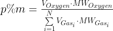
I used a table from the Wikipedia and did the Equation 1 calculation as illustrated in Figure 2.

Figure 2: Calculating the Percentage of Oxygen in the Atmosphere by Mass.

Figure 2: Calculating the Percentage of Oxygen in the Atmosphere by Mass.

Mass of Oxygen in the Atmosphere

Figure 3 shows the calculation for the total mass of oxygen in today's atmosphere.

Figure 3: Calculating the Mass of Oxygen in the Atmosphere.

Figure 3: Calculating the Mass of Oxygen in the Atmosphere.

Conclusion

Let's see if I can check my answers. According to the National Center for Atmospheric Research, the total mass of the Earth's atmosphere is 5.1353·1015 metric tons. So I have good agreement there. My estimate for the mass fraction of oxygen in the Earth's atmosphere (23.1%) equals that stated in the Wikipedia, so I am good there. My estimate for the total mass of O2 in the atmosphere is 1.2 million billion metric tons, which agrees with this reference. So overall the analysis is pretty close.

The stromatolites alone produced 20 million billion tons (possibly more, see Appendix). The majority of the oxygen produced by stromatolites has apparently gone somewhere other than the atmosphere. In fact, there are enormous amounts of atmospheric oxygen that ended up chemically tied up in rocks. Consider the following quote (Source).

While photosynthetic life reduced the carbon dioxide content of the atmosphere, it also started to produce oxygen. For a long time, the oxygen produced did not build up in the atmosphere, since it was taken up by rocks, as recorded in Banded Iron Formations (BIFs) and continental red beds. To this day, the majority of oxygen produced over time is locked up in the ancient "banded rock" and "red bed" formations. It was not until probably only 1 billion years ago that the reservoirs of oxidizable rock became saturated and the free oxygen stayed in the air.

Figure 4 is from the Wikipedia and does a nice job illustrating the Earth's O2 level over time. The red and green lines illustrate the range of estimates for the percentage of O2.

Figure 4:Earth's Atmospheric Oxygen Percentage Versus Time.

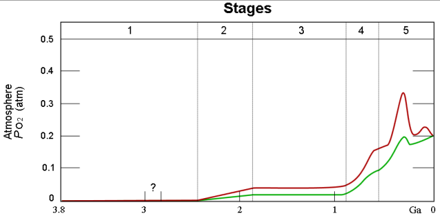
Figure 4: Earth's Atmospheric Oxygen Percentage Versus Time.

There are some folks that claim the high oxygen levels in the past may have played a role in making dinosaurs so large.

Appendix A: Interesting Quote on Stromatolite-Produced Oxygen

Figure 5 shows where the photosynthesized oxygen went (Source). Note that this reference assumes that the total amount of photosynthesized mass of O2 on Earth is 3x10²² grams (=30 million billion metric tons). Clearly, estimates for the amount of photosynthesized O2 vary a bit.

Figure 5: Cumulative History of O2 by Photosynthesis Through Geologic Time.

Figure 5: Cumulative History of O2 by Photosynthesis Through Geologic Time.

The following quote (source) describes how most of the oxygen was chemically bound to the Earth and the rest was released to the air.

A sort of mass balance for atmospheric oxygen (including that dissolved in the sea) is shown in Figure 13.8 [my Figure 5]. The excess oxygen depends on a corresponding accumulation of organic matter (plus biologically reduced sulphur and methane) that has become buried in sedimentary deposits. About 58% and 38% of this oxygen has been used for the oxidation of iron and sulphur, respectively during the 3.5 - 3.8 billion years of organic photosynthesis. The remaining 4% (about 1.2x10¹⁵ tonnes) is found as free O2. The turnover rate of this atmospheric oxygen is only about 4000 years and is caused by organic photosynthesis and respiration processes that almost balance so that the biological turnover is vastly faster than the slow accumulation of organic matter. Given the crude estimates in Figure 13.5. there is altogether an excess of 3x10¹⁶ tonnes of oxygen (of which the greater part is in the form of oxidized iron and sulphur and only 4% as O2). Over roughly four billion years this corresponds to a net accumulation of 7.7x10⁶ tonnes per year. The annual turnover due to photosynthesis and respiration corresponds to (1.2x10¹⁵[tonnes])/4000 [years] = 3x10¹⁰[11] tonnes O2 per year; that is production and respiration is about 20,000[36,500] times faster than the slow accumulation of organic matter in sedimentary rocks. This calculation, of course, assumes that both the production rate and the rate of accumulation of un-mineralized organic matter have been constant over geological time. Some evidence indicates that this has been the case since roughly the second half of the Precambrian.

As you can see from the quote, the calculation of total O2 production over the history of the Earth requires a number of assumptions.

I have noticed some minor math errors (see highlights) in the quote given above – minor in the sense that they do not change the result qualitatively, but I do see some calculation issues. Figure 6 shows my version of the calculations using the data given above. In the calculation, I assume that the period of organic photosynthesis was 3.65 billion years (the mean of the range given in the quote).

Detailed Calculation Using Given Data.

Figure 6: Detailed Calculation Using Given Data.

Save

Posted in General Science, History of Science and Technology | 15 Comments

Star Trek Analogies to Engineering Management

It amazes me how often my management experiences remind me of Star Trek episodes. A good example came up today. At extremely regular intervals, I must prepare budget reports that document the spending of my department. If I am late, I receive emails that progressively get nastier until I feed the accounting monster. While preparing this budget report today, one of my senior engineers asked me what I was doing. I told him that I was feeding Vaal. For the uninitiated, Vaal is a machine from Star Trek that a group of primitive people were obligated to bring food to every day. A loud bong is struck when Vaal needs to be fed. When Vaal was denied food for any significant length of time, he got really nasty (e.g. generated storms, threw lightning bolts, etc). The analogy is just too good.

Figure 1: Vaal from Star Trek. Its behavior is similar to that of my budget minders.

Figure 1: Vaal from Star Trek. Its behavior is similar to that of my budget minders.

Posted in Management | 1 Comment

Battery State of Charge

Introduction

Nearly all of our products are sold with an Uninterruptable Power Supply (UPS) because customers need phone service for emergency voice calls, which we refer to as "lifeline service". Batteries are used for energy storage in all of our UPS hardware we sell. I do not know a single engineer who regularly deals with batteries that likes them. They are the biggest pain I deal with. Here is my summary of complaints:

  • They are expensive.
    Batteries often contain materials that are very expensive. Battery cost is strongly affected by commodity prices. It was not long ago that a commodity price bubble caused me great pain as I tried to keep my unit product cost down.
  • They require replacement at regular intervals (every 3 to 5 years) to ensure they work when needed
  • There are always safety issues to address
    Look at the history of Li-ion batteries and their tendency to catch fire. Many battery chemistries emit explosive gases (e.g. lead-acid batteries emit hydrogen when being charged).
  • They often contain materials that are expensive to dispose of.
    Batteries often contain materials like lead (e.g. lead-acid batteries) or cadmium (eg. Nicad batteries). These are poisonous elements that are expensive to dispose of safely.
  • Charging is often a complicated operation.
  • Battery performance is strongly temperature dependent.

Our UPS vendor has a "low battery" alarm that supposedly tells the customer when the battery capacity has been reduced to 20% of its rating. This is an extremely deceptive alarm. I have spent much time trying to accurately predict remaining battery capacity and have not been totally successful. This is a complicated question because a battery is a chemical beast that is subject to temperature and aging effects that make accurate prediction of it remaining capacity difficult.

Today, our customer service group asked me to explain what "20% capacity remaining" really means. All I could do was sigh and give the following answer.

Analysis

Most UPS hardware tries to estimate their battery's state of charge by measuring the battery terminal voltage. Figure 1 shows the terminal voltage versus state of charge voltage for a 6-cell, 12 V lead-acid battery.

Figure 1: Battery Terminal Voltage (V) Versus State of Charge (%).

Figure 1: Battery Terminal Voltage (V) Versus State of Charge (%).


People unfamiliar with batteries see that there are multiple curves that are labeled with things like "C/100" or "C/3". These curves represent the current load the battery is under load. The ratio "C/T" represents represents the capacity of the battery in amp-hours (C) and the discharge time (T).

Eq. 1 I_{Discharge}=\frac{C}{T_{Discharge}}

where C is the battery capacity in amp-hours and TDischarge is the discharge time.

The UPS we use has its low battery alarm set to activate when the terminal voltage drops below 11.0 V. However, an 11.0 V terminal voltage only represents 20% capacity when the battery load is C/5. In my application, the load is C/10. This means that in my application the low battery alarms is asserted when the battery is almost completely discharged. This has caused some issues for customers who want to depend on that last 20%. Unfortunately, they cannot depend on that battery having any capacity left when the low battery alarm is activated.

Temperature also complicates the situation. Everything I have said above assumes a temperature of 77 °F (25 °C). Battery capacity depends strongly on temperature, which is shown by Figure 2.

Figure 2: Battery Capacity Variation with Temperature.

Figure 2: Battery Capacity Variation with Temperature.


If your UPS is at a temperature other than 77 °F, you will need to compensate for the temperature variation.

Battery capacity is also a function of the age and charging history of the battery. Older batteries do not have as much capacity as new batteries because of corrosion effects. Batteries that have been through many charge and discharge cycles have less capacity than new batteries because battery capacity degrades with each discharge/charge cycle.

Conclusion

Accurately predicting reserve battery capacity is a complicated thing. I try to avoid it whenever I can.

Posted in Batteries, Electronics | Comments Off on Battery State of Charge

Quotes of the Day

Since I began sending emails, I have put quotes at the bottom of them. I change the quote for every email I send. Many people have said that they enjoy them. I thought I would include the most popular here.

Quote Source Quote
A spacecraft designer whose name I don't recall. I don't believe there is intelligent life on other planets. I believe they are just like us.
Professor J.A. Young ... no important contribution was ever first conceived in a manner consistent with what was then known factually -- otherwise someone else could have made the contribution earlier ... In each instance, someone had to make a wild leap -- to his credit (since we tend to forget the 'crackpots' who did the same and missed) ... This ... attitude should be transmitted ... This is the poetry of science.
Admiral Rickover, 1983, commenting on how changing a failing school is one of the most difficult challenges around. Changing schools is like moving a graveyard.
Lord Rutherford All science is either physics or stamp collecting.
The Lenten sacrifice of an engineer. I am going to give up Pilsners.
Petronious Arbiter, 210 BC We trained hard, but it seemed that every time we were beginning to form up into teams, we would be reorganized. I was to learn later in life that we tend to meet any new situation by reorganizing; and a wonderful method it can be for creating the illusion of progress while producing confusion, inefficiency, and demoralization.
Roald Amundsen (1872-1928), first man to the South Pole. He is considered by many to have been the most efficient of the great explorers. Adventure is just bad planning.
Russian story of a mathematician. There is a story. A balloon floats away in the clouds. The crew caught sight of a man and shouted to him 'Where are we?' The man replies 'You are in a basket.' It was an answer of a mathematician. Only a mathematician could give an absolutely right and absolutely useless answer.
Scientist on the differences between engineers and scientist. Surprises - they are the difference between engineers and scientists. Engineers hate surprises. We love them.
Tom Wescott, control systems engineer on how helicopters fly. Helicopters fly by vibrating so hard that some components exceed the speed of light. This causes an anti-gravity effect that makes the helicopter lift off the ground. The blades are just there for control. This high vibration environment can be bad on electronics, particularly if some of their sensitive components are the ones exceeding the speed of light.
Pamela Anderson I don’t really think about anything too much. I live in the present. I move on. I don’t think about what happened yesterday. If I think too much, it kind of freaks me out.
My mother on religion. You'd better pray that will come out of that carpet!
My mother on safety. You fall out of that tree and break both your legs, don't come running home to me.
Teddy Roosevelt, answering a press question about his wild eldest daughter Alice. Alice was an early version of the Bush twins. I can be President of the United States or I can control Alice. I cannot possibly do both.
Posted in Personal | Comments Off on Quotes of the Day

Super Full Moon

One of the engineers just stopped by and told me that Saturday (19-Mar-2011) we will have a "Super Full Moon". This means we will have a full moon and it will be unusually large (14% wider). See this link for details. I will have to get out Saturday night and take a look.

Posted in Astronomy | 1 Comment

Dimensional Analysis and Olympic Rowing

Introduction

I have always found dimensional analysis to be a very useful engineering tool. I recently watched a video Professor John Barrow of Gresham College who did a very nice job illustrating how dimensional analysis can be used to derive useful results. One example that particularly intrigued me involved Olympic rowing. Using dimensional analysis, he was able to derive a relationship between the crew size of a rowboat and its speed. He then curve fit the results from the 1980 Olympics to his relationship and showed that for one Olympic year there was good agreement. I thought it would be a good illustration of the power of Mathcad's curve fitting routines to show how easy it is to extend this analysis to multiple Olympic years.

Background

I am not a rower, but I will summarize the small amount that I needed to know to model rowboat velocity versus the number of rowers.

  • Coxless Versus Coxed
    The crews of rowboats consists of rowers and an optional coxswain (often shortened to cox). The cox will steer and keep the pace.
  • Course Length
    Races are over a 2000 meter course.
  • Crew sizes
    For this exercise, I will be looking at coxless gold medal scores with 1, 2, or 4 male rowers. I will also examine coxed gold medal scores for 2,4, and 8 male rower crews.
  • Speed Calculation
    I will be looking at over speed, v, over the course, which I compute using v = \frac{d}{t}.

Analysis

While I recommend Professor Barrow's lecture for the details of showing that rowboat velocity increases with the 9th root of the number of rower, I do summarize his derivation in Equation 1. It is terse, but you can get the gist of the argument.

Eq. 1 {{F}_{Drag}}\propto {{v}^{2}}\cdot {{A}_{Wetted}}
P={{F}_{Drag}}\cdot v\Rightarrow P\propto \left( {{v}^{2}}\cdot {{A}_{Wetted}} \right)\cdot v
P={{N}_{Rowers}}\cdot {{P}_{Rower}}\Rightarrow N\propto {{v}^{3}}\cdot {{A}_{Wetted}}
By Archimedes law, displaced volume increases linearly with the number of rowers. This means the wetted area increases by the 2/3 power of the number of rowers.
{{A}_{Wetted}}\propto N_{Rowers}^{\frac{2}{3}}
{{N}_{Rowers}}\propto {{v}^{3}}\cdot N_{Rowers}^{\frac{2}{3}}
\therefore v\propto N_{Rowers}^{\frac{1}{9}}

A similar derivation is shown in Equation 2 for a coxed rowboat, assuming the cox weights half that of a rower.

Eq. 2 {{F}_{Drag}}\propto {{v}^{2}}\cdot {{A}_{Wetted}}
P={{F}_{Drag}}\cdot v\Rightarrow P\propto \left( {{v}^{2}}\cdot {{A}_{Wetted}} \right)\cdot v
P={{N}_{Rowers}}\cdot {{P}_{Rower}}\Rightarrow N\propto {{v}^{3}}\cdot {{A}_{Wetted}}
{{A}_{Wetted}}\propto \left( N+0.5 \right)_{Rowers}^{\frac{2}{3}}
{{N}_{Rowers}}\propto {{v}^{3}}\cdot \left( N+0.5 \right)_{Rowers}^{\frac{2}{3}}
\therefore v\propto \frac{{{N}^{\frac{1}{3}}}}{\left( N+0.5 \right)_{Rowers}^{\frac{2}{9}}}

Coxless Rowing (Equation 1)

I will now use Mathcad to fit Olympic rowing data to the 9th root curve. Figure 1 summarizes my results for the Olympic gold medal results of 1976, 1980, and 1984 for coxless 1, 2, and 4 man rowboats.

Figure 1: Coxless Rowing Analysis Results.

Figure 1: Coxless Rowing Analysis Results.

Coxed Rowing (Equation 2)

The difference between Equations 1 and 2 is that cox adds weight and no power. I will now use Mathcad to fit Olympic rowing data to Equation 2. Figure 1 summarizes my results for the Olympic gold medal results of 1976, 1980, and 1984 for coxed 2, 4, and 8 man rowboats.

Figure 2: Coxed Rowing Analysis Results.

Figure 2: Coxed Rowing Analysis Results.

Conclusion

Considering the crudeness of the model, the results were not too bad. It was a nice use of dimensional analysis to gain insight into a problem. The main issue I have with the model lies in the estimate of the wetted surface area. But Professor Barrow's approach is a great first-order approximation. If I was looking for improvements, I might look closer at that wetted surface area equation.

Posted in General Mathematics | 1 Comment

A Little Drive-By Math Incident

A quick math problem came by my cube today that was worth sharing. I was asked if there was a closed-form solution to Equation 1.

Eq. 1 \ln ({{x}^{x}})=4

This problem does not have a closed form solution using the "everyday" functions, but it is solvable using Lambert's W function. Recall that Lambert's W function has the property shown in Equation 2.

Eq. 2 z~=~W\left( z \right)\cdot {{e}^{W(z)}}

We can hammer equation 1 into the form of Equation 2 by the process shown in Equation 3.

Eq. 3 x\cdot \ln (x)=4
{{e}^{\ln (x)}}\cdot \ln (x)=4
{{e}^{W(4)}}\cdot W(4)=4
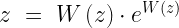
, definition of W function
\text{Let }W(4)=\ln (x)
\therefore x={{e}^{W(4)}}

We now have a closed form solution, but it requires the use of a relatively uncommon function. Let's compute the numeric solution. As shown in Figure 1, I drop into Mathcad for this part.

Figure 1: Numerical Solution in Mathcad.

Figure 1: Numerical Solution in Mathcad.

Posted in General Mathematics | Comments Off on A Little Drive-By Math Incident

Trigonometry, WWII Torpedoes, and a Museum Docent

Introduction

I received a message a few weeks ago from a docent at an East Coast museum. He was using an article I wrote for the Wikipedia years ago to demonstrate an application of trigonometry to high school kids. In that article, there was a figure that had a typo in it and he wanted it corrected so he could use it for his class. Since my Wikipedia writings have primarily been about military history, I was a bit surprise that he was using material I created to teach trigonometry. We traded some emails, I corrected the typo, and what he was doing turned out to be interesting. I decided it was worth covering here.

Background

The Wikipedia article I had written was about torpedo fire control during World War II. The docent was creating a simulation of World War II submarine combat in an effort to provide an exciting experience for kids that involved history and trigonometry – two of my favorite subjects. The kids would be able to get a feel for the difficulty of what their great-grandfathers were trying to do nearly 70 years ago. It's always fun trying to explain what they would have to go through to calculate the measurements needed. It often startles them to learn that it wasn't as simple as using a calculator to aid them with their calculations. Calculators weren't created until the 1960s, and even then you wouldn't be able to search for graphing calculators reviews by bestcalculators.net since the internet didn't exist either. You would have to work out everything you needed by hand and mental math. So, understanding trigonometry was paramount to make sure your calculation wasn't incorrect.

To understand the fire control problem, we need to define some terms. Figure 1 provides a visual illustration of the World War II torpedo fire control variables.

Figure 1: Definition of Torpedo Fire Control Terms.

Figure 1: Definition of Torpedo Fire Control Terms.


It turns out, that Figure 1 also illustrates the fire control problem. Equation 1 shows the equation that World War II sub skippers had to solve. If you look closely, it is a restatement of the law of sines.

Eq. 1 \frac{\left\| {{v}_{Target}} \right\|}{\sin ({{\theta }_{Deflection}})}=\frac{\left\| {{v}_{Torpedo}} \right\|}{\sin ({{\theta }_{Bow}})}
substitute {{\theta }_{Bow}}~={{\theta }_{Track}}-{{\theta }_{Deflection}}
\therefore \frac{\left\| {{v}_{Target}} \right\|}{\sin ({{\theta }_{Deflection}})}=\frac{\left\| {{v}_{Torpedo}} \right\|}{\sin ({{\theta }_{Track}}-{{\theta }_{Deflection}})}
  • vTarget is the velocity of the target.
  • vTorpedo is the velocity of the torpedo.
  • ?Bow is the angle of the target ship bow relative to the target bearing.
  • ?Deflection is the angle of the torpedo course relative to the target bearing and is the critical value we are computing here.
  • ?Track is the angle between the target ship's course and the torpedo's course.

These old torpedoes ran on a straight line that was determined by the \theta_{Gyro} 
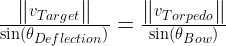
angle, which we compute using Equation 2.

Eq. 2 {{\theta }_{Gyro}}={{\theta }_{Bearing}}-{{\theta }_{Deflection}}

where \theta_{Bearing} is read from the submarine's compass and \theta_{Deflection} was computed by the Torpedo Data Computer (TDC), an analog computer built to solve Equation 1.

Just like the TDC, we can solve Equation 1 for {{\theta }_{Deflection}} versus {{\theta }_{Track}} to generate Figure 2. This is the figure that had the typo the docent wanted corrected. The typo of my original figure was in the equation that I had included as a note.

Figure 2: Torpedo Track Angle Versus Deflection Angle.

Figure 2: Torpedo Track Angle Versus Deflection Angle.


I originally saw this curve in the Submarine Torpedo Fire Control Manual. Sub skippers were told to try to fire with track angles at the optimum values, which are marked by small triangles in Figure 2. It was difficult for sub skippers to get an accurate estimate of the target ship's course {{\theta }_{Bow}}, which was used to compute {{\theta }_{Track}}. The optimum track angle is where the {{\theta }_{Deflection}} curve is flat, which means that the impact of errors in {{\theta }_{Track}} are minimized.

Conclusion

You never know where your work will turn up. When the docent finishes his simulation, I am going to travel to the East Coast and try it out.

If you are wondering how I ever got interested in this subject, it is a long story that goes back to my childhood. One critical part of the story involves the book "Clear the Bridge" by Richard O'Kane. I consider that book the finest description of World War II submarine combat that I have ever read (and I read them all). Admiral O'Kane's writing has a lively style that made quite an impression on a teenage boy.

Posted in History of Science and Technology, Underwater | 8 Comments

Neat Pictures from Mars and the Moon

One of my favorite blogs is written by Emily Lakadawalla for the Planetary Society. I was looking at some of her old material and found some pictures that I had never seen and I thought I would share with my readers. Figure 1 is a photograph of the Spirit rover taken by the Mars Reconnaissance Orbiter using the HiRISE camera. This is just amazing.

Figure 1: Spirit Rover on Mars.

Figure 1: Spirit Rover on Mars.


While reading Emily's blog, I got to wondering if there were any photographs of the landing sites on the Moon. A quick Google search that NASA has done its usual good job of making some great images available. Figure 2 shows the Apollo 11 landing site.
Figure 2: Apollo 11 Landing Site.

Figure 2: Apollo 11 Landing Site.


Figure 3 shows the Apollo 14 landing site.
Figure 3: Apollo 14 Landing Site.

Figure 3: Apollo 14 Landing Site.


These pictures have been around for awhile, but they were new to me! I think they are great.

Posted in Astronomy | 1 Comment