Quotes of the Day

Since I began sending emails, I have put quotes at the bottom of them. I change the quote for every email I send. Many people have said that they enjoy them. I thought I would include the most popular here.

Quote Source Quote
A spacecraft designer whose name I don't recall. I don't believe there is intelligent life on other planets. I believe they are just like us.
Professor J.A. Young ... no important contribution was ever first conceived in a manner consistent with what was then known factually -- otherwise someone else could have made the contribution earlier ... In each instance, someone had to make a wild leap -- to his credit (since we tend to forget the 'crackpots' who did the same and missed) ... This ... attitude should be transmitted ... This is the poetry of science.
Admiral Rickover, 1983, commenting on how changing a failing school is one of the most difficult challenges around. Changing schools is like moving a graveyard.
Lord Rutherford All science is either physics or stamp collecting.
The Lenten sacrifice of an engineer. I am going to give up Pilsners.
Petronious Arbiter, 210 BC We trained hard, but it seemed that every time we were beginning to form up into teams, we would be reorganized. I was to learn later in life that we tend to meet any new situation by reorganizing; and a wonderful method it can be for creating the illusion of progress while producing confusion, inefficiency, and demoralization.
Roald Amundsen (1872-1928), first man to the South Pole. He is considered by many to have been the most efficient of the great explorers. Adventure is just bad planning.
Russian story of a mathematician. There is a story. A balloon floats away in the clouds. The crew caught sight of a man and shouted to him 'Where are we?' The man replies 'You are in a basket.' It was an answer of a mathematician. Only a mathematician could give an absolutely right and absolutely useless answer.
Scientist on the differences between engineers and scientist. Surprises - they are the difference between engineers and scientists. Engineers hate surprises. We love them.
Tom Wescott, control systems engineer on how helicopters fly. Helicopters fly by vibrating so hard that some components exceed the speed of light. This causes an anti-gravity effect that makes the helicopter lift off the ground. The blades are just there for control. This high vibration environment can be bad on electronics, particularly if some of their sensitive components are the ones exceeding the speed of light.
Pamela Anderson I don’t really think about anything too much. I live in the present. I move on. I don’t think about what happened yesterday. If I think too much, it kind of freaks me out.
My mother on religion. You'd better pray that will come out of that carpet!
My mother on safety. You fall out of that tree and break both your legs, don't come running home to me.
Teddy Roosevelt, answering a press question about his wild eldest daughter Alice. Alice was an early version of the Bush twins. I can be President of the United States or I can control Alice. I cannot possibly do both.
Posted in Personal | Comments Off on Quotes of the Day

Super Full Moon

One of the engineers just stopped by and told me that Saturday (19-Mar-2011) we will have a "Super Full Moon". This means we will have a full moon and it will be unusually large (14% wider). See this link for details. I will have to get out Saturday night and take a look.

Posted in Astronomy | 1 Comment

Dimensional Analysis and Olympic Rowing

Introduction

I have always found dimensional analysis to be a very useful engineering tool. I recently watched a video Professor John Barrow of Gresham College who did a very nice job illustrating how dimensional analysis can be used to derive useful results. One example that particularly intrigued me involved Olympic rowing. Using dimensional analysis, he was able to derive a relationship between the crew size of a rowboat and its speed. He then curve fit the results from the 1980 Olympics to his relationship and showed that for one Olympic year there was good agreement. I thought it would be a good illustration of the power of Mathcad's curve fitting routines to show how easy it is to extend this analysis to multiple Olympic years.

Background

I am not a rower, but I will summarize the small amount that I needed to know to model rowboat velocity versus the number of rowers.

  • Coxless Versus Coxed
    The crews of rowboats consists of rowers and an optional coxswain (often shortened to cox). The cox will steer and keep the pace.
  • Course Length
    Races are over a 2000 meter course.
  • Crew sizes
    For this exercise, I will be looking at coxless gold medal scores with 1, 2, or 4 male rowers. I will also examine coxed gold medal scores for 2,4, and 8 male rower crews.
  • Speed Calculation
    I will be looking at over speed, v, over the course, which I compute using v = \frac{d}{t}.

Analysis

While I recommend Professor Barrow's lecture for the details of showing that rowboat velocity increases with the 9th root of the number of rower, I do summarize his derivation in Equation 1. It is terse, but you can get the gist of the argument.

Eq. 1 {{F}_{Drag}}\propto {{v}^{2}}\cdot {{A}_{Wetted}}
P={{F}_{Drag}}\cdot v\Rightarrow P\propto \left( {{v}^{2}}\cdot {{A}_{Wetted}} \right)\cdot v
P={{N}_{Rowers}}\cdot {{P}_{Rower}}\Rightarrow N\propto {{v}^{3}}\cdot {{A}_{Wetted}}
By Archimedes law, displaced volume increases linearly with the number of rowers. This means the wetted area increases by the 2/3 power of the number of rowers.
{{A}_{Wetted}}\propto N_{Rowers}^{\frac{2}{3}}
{{N}_{Rowers}}\propto {{v}^{3}}\cdot N_{Rowers}^{\frac{2}{3}}
\therefore v\propto N_{Rowers}^{\frac{1}{9}}

A similar derivation is shown in Equation 2 for a coxed rowboat, assuming the cox weights half that of a rower.

Eq. 2 {{F}_{Drag}}\propto {{v}^{2}}\cdot {{A}_{Wetted}}
P={{F}_{Drag}}\cdot v\Rightarrow P\propto \left( {{v}^{2}}\cdot {{A}_{Wetted}} \right)\cdot v
P={{N}_{Rowers}}\cdot {{P}_{Rower}}\Rightarrow N\propto {{v}^{3}}\cdot {{A}_{Wetted}}
{{A}_{Wetted}}\propto \left( N+0.5 \right)_{Rowers}^{\frac{2}{3}}
{{N}_{Rowers}}\propto {{v}^{3}}\cdot \left( N+0.5 \right)_{Rowers}^{\frac{2}{3}}
\therefore v\propto \frac{{{N}^{\frac{1}{3}}}}{\left( N+0.5 \right)_{Rowers}^{\frac{2}{9}}}

Coxless Rowing (Equation 1)

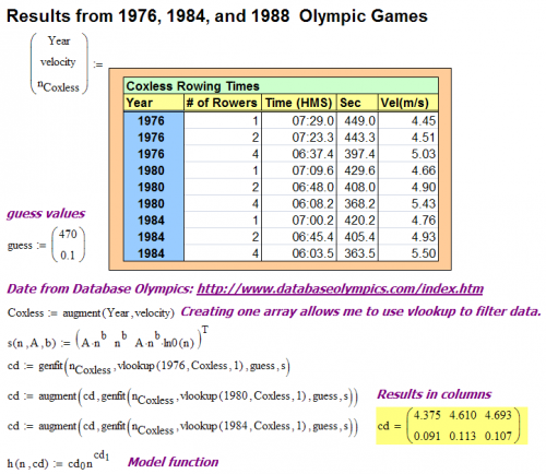
I will now use Mathcad to fit Olympic rowing data to the 9th root curve. Figure 1 summarizes my results for the Olympic gold medal results of 1976, 1980, and 1984 for coxless 1, 2, and 4 man rowboats.

Figure 1: Coxless Rowing Analysis Results.

Figure 1: Coxless Rowing Analysis Results.

Coxed Rowing (Equation 2)

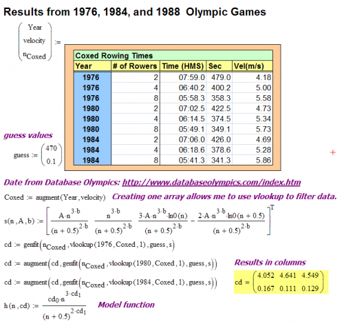
The difference between Equations 1 and 2 is that cox adds weight and no power. I will now use Mathcad to fit Olympic rowing data to Equation 2. Figure 1 summarizes my results for the Olympic gold medal results of 1976, 1980, and 1984 for coxed 2, 4, and 8 man rowboats.

Figure 2: Coxed Rowing Analysis Results.

Figure 2: Coxed Rowing Analysis Results.

Conclusion

Considering the crudeness of the model, the results were not too bad. It was a nice use of dimensional analysis to gain insight into a problem. The main issue I have with the model lies in the estimate of the wetted surface area. But Professor Barrow's approach is a great first-order approximation. If I was looking for improvements, I might look closer at that wetted surface area equation.

Posted in General Mathematics | 1 Comment

A Little Drive-By Math Incident

A quick math problem came by my cube today that was worth sharing. I was asked if there was a closed-form solution to Equation 1.

Eq. 1 \ln ({{x}^{x}})=4

This problem does not have a closed form solution using the "everyday" functions, but it is solvable using Lambert's W function. Recall that Lambert's W function has the property shown in Equation 2.

Eq. 2 z~=~W\left( z \right)\cdot {{e}^{W(z)}}

We can hammer equation 1 into the form of Equation 2 by the process shown in Equation 3.

Eq. 3 x\cdot \ln (x)=4
{{e}^{\ln (x)}}\cdot \ln (x)=4
{{e}^{W(4)}}\cdot W(4)=4, definition of W function
\text{Let }W(4)=\ln (x)
\therefore x={{e}^{W(4)}}

We now have a closed form solution, but it requires the use of a relatively uncommon function. Let's compute the numeric solution. As shown in Figure 1, I drop into Mathcad for this part.

Figure 1: Numerical Solution in Mathcad.

Figure 1: Numerical Solution in Mathcad.

Posted in General Mathematics | Comments Off on A Little Drive-By Math Incident

Trigonometry, WWII Torpedoes, and a Museum Docent

Introduction

I received a message a few weeks ago from a docent at an East Coast museum. He was using an article I wrote for the Wikipedia years ago to demonstrate an application of trigonometry to high school kids. In that article, there was a figure that had a typo in it and he wanted it corrected so he could use it for his class. Since my Wikipedia writings have primarily been about military history, I was a bit surprise that he was using material I created to teach trigonometry. We traded some emails, I corrected the typo, and what he was doing turned out to be interesting. I decided it was worth covering here.

Background

The Wikipedia article I had written was about torpedo fire control during World War II. The docent was creating a simulation of World War II submarine combat in an effort to provide an exciting experience for kids that involved history and trigonometry – two of my favorite subjects. The kids would be able to get a feel for the difficulty of what their great-grandfathers were trying to do nearly 70 years ago. It's always fun trying to explain what they would have to go through to calculate the measurements needed. It often startles them to learn that it wasn't as simple as using a calculator to aid them with their calculations. Calculators weren't created until the 1960s, and even then you wouldn't be able to search for graphing calculators reviews by bestcalculators.net since the internet didn't exist either. You would have to work out everything you needed by hand and mental math. So, understanding trigonometry was paramount to make sure your calculation wasn't incorrect.

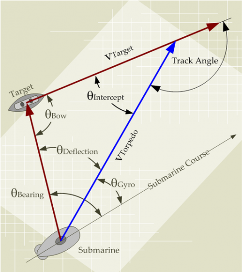
To understand the fire control problem, we need to define some terms. Figure 1 provides a visual illustration of the World War II torpedo fire control variables.

Figure 1: Definition of Torpedo Fire Control Terms.

Figure 1: Definition of Torpedo Fire Control Terms.


It turns out, that Figure 1 also illustrates the fire control problem. Equation 1 shows the equation that World War II sub skippers had to solve. If you look closely, it is a restatement of the law of sines.

Eq. 1 \frac{\left\| {{v}_{Target}} \right\|}{\sin ({{\theta }_{Deflection}})}=\frac{\left\| {{v}_{Torpedo}} \right\|}{\sin ({{\theta }_{Bow}})}
substitute {{\theta }_{Bow}}~={{\theta }_{Track}}-{{\theta }_{Deflection}}
\therefore \frac{\left\| {{v}_{Target}} \right\|}{\sin ({{\theta }_{Deflection}})}=\frac{\left\| {{v}_{Torpedo}} \right\|}{\sin ({{\theta }_{Track}}-{{\theta }_{Deflection}})}
  • vTarget is the velocity of the target.
  • vTorpedo is the velocity of the torpedo.
  • ?Bow is the angle of the target ship bow relative to the target bearing.
  • ?Deflection is the angle of the torpedo course relative to the target bearing and is the critical value we are computing here.
  • ?Track is the angle between the target ship's course and the torpedo's course.

These old torpedoes ran on a straight line that was determined by the \theta_{Gyro} angle, which we compute using Equation 2.

Eq. 2 {{\theta }_{Gyro}}={{\theta }_{Bearing}}-{{\theta }_{Deflection}}

where \theta_{Bearing} is read from the submarine's compass and \theta_{Deflection} was computed by the Torpedo Data Computer (TDC), an analog computer built to solve Equation 1.

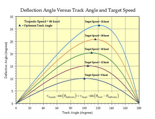
Just like the TDC, we can solve Equation 1 for {{\theta }_{Deflection}} versus {{\theta }_{Track}} to generate Figure 2. This is the figure that had the typo the docent wanted corrected. The typo of my original figure was in the equation that I had included as a note.

Figure 2: Torpedo Track Angle Versus Deflection Angle.

Figure 2: Torpedo Track Angle Versus Deflection Angle.


I originally saw this curve in the Submarine Torpedo Fire Control Manual. Sub skippers were told to try to fire with track angles at the optimum values, which are marked by small triangles in Figure 2. It was difficult for sub skippers to get an accurate estimate of the target ship's course {{\theta }_{Bow}}, which was used to compute {{\theta }_{Track}}. The optimum track angle is where the {{\theta }_{Deflection}} curve is flat, which means that the impact of errors in {{\theta }_{Track}} are minimized.

Conclusion

You never know where your work will turn up. When the docent finishes his simulation, I am going to travel to the East Coast and try it out.

If you are wondering how I ever got interested in this subject, it is a long story that goes back to my childhood. One critical part of the story involves the book "Clear the Bridge" by Richard O'Kane. I consider that book the finest description of World War II submarine combat that I have ever read (and I read them all). Admiral O'Kane's writing has a lively style that made quite an impression on a teenage boy.

Posted in History of Science and Technology, Underwater | 8 Comments

Neat Pictures from Mars and the Moon

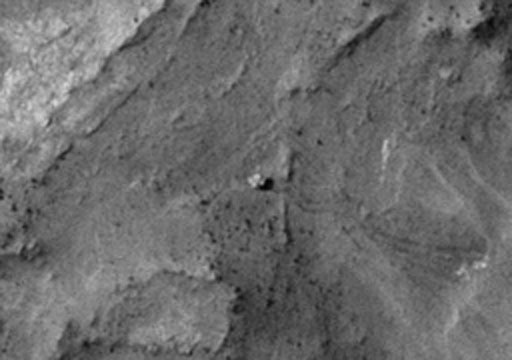
One of my favorite blogs is written by Emily Lakadawalla for the Planetary Society. I was looking at some of her old material and found some pictures that I had never seen and I thought I would share with my readers. Figure 1 is a photograph of the Spirit rover taken by the Mars Reconnaissance Orbiter using the HiRISE camera. This is just amazing.

Figure 1: Spirit Rover on Mars.

Figure 1: Spirit Rover on Mars.


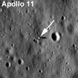
While reading Emily's blog, I got to wondering if there were any photographs of the landing sites on the Moon. A quick Google search that NASA has done its usual good job of making some great images available. Figure 2 shows the Apollo 11 landing site.
Figure 2: Apollo 11 Landing Site.

Figure 2: Apollo 11 Landing Site.


Figure 3 shows the Apollo 14 landing site.
Figure 3: Apollo 14 Landing Site.

Figure 3: Apollo 14 Landing Site.


These pictures have been around for awhile, but they were new to me! I think they are great.

Posted in Astronomy | 1 Comment

Current Source Built with a Negative Resistance

Introduction

I have seen quite a few schematics lately that are using an operational amplifier (opamp) configured as a negative resistor. I thought it would be interesting to analyze this circuit and show how it can provide an economical solution to a common sensor interface scenario.

Background

Figure 1 illustrates a common sensor interface scenario. This scenario consists of:

  • Sensor
    The sensor has a resistance characteristic that varies according to some external parameter, e.g. temperature, ambient light level, gas concentration.
  • Current Source
    A current source drive can be desirable for a number of reasons: (1) The sensor may be calibrated for a specific current level, (2) The sensor may have a linear response for a given current drive, (3) The sensor output voltage range needs to be restricted in some way.
  • Amplifier
    The amplifier is often needed to provide isolation from the monitoring circuitry and to scale the output for further signal processing.
Figure 1: Common Sensor Interface Scenario.

Figure 1: Common Sensor Interface Scenario.

Negative Resistance Opamp Circuit

Figure 2 shows an operational amplifier connected as a negative resistance.

Figure 2: Negative Resistance Circuit.

Figure 2: Negative Resistance Circuit.

Equation 1 shows the derivation of the negative resistance equation.

Eq. 1 {{v}_{I}}={{v}_{O}}+i\cdot {{R}_{F}}
{{v}_{I}}={{v}_{O}}\cdot \frac{{{R}_{1}}}{{{R}_{1}}+{{R}_{2}}}
{{v}_{I}}={{v}_{I}}\cdot \frac{{{R}_{1}}+{{R}_{2}}}{{{R}_{1}}}+i\cdot {{R}_{F}}
-{{v}_{I}}\cdot \frac{{{R}_{2}}}{{{R}_{1}}}=i\cdot {{R}_{F}}\Rightarrow {{Z}_{IN}}\triangleq \frac{{{v}_{I}}}{i}=-{{R}_{F}}\cdot \frac{{{R}_{1}}}{{{R}_{2}}}

Equation 2 shows the derivation of the voltage gain equation.

Eq. 2 {{v}_{I}}={{v}_{O}}\cdot \frac{{{R}_{1}}}{{{R}_{1}}+{{R}_{2}}}\Rightarrow {{A}_{v}}\triangleq \frac{{{v}_{O}}}{{{v}_{I}}}=\frac{{{R}_{1}}+{{R}_{2}}}{{{R}_{1}}}

Introduction

My application example is shown in Figure 4.

Figure 3: Negative Resistance Example Application.

Figure 3: Negative Resistance Example Application.


The basic idea here is to use negative input resistance of the opamp circuit to cancel out the resistance of RS. Figure 4 illustrates this source transformation.
Figure 4: Source Transformation.

Figure 4: Source Transformation.


The parameters of this case are the following:

  • V_{CC} = 10 V
  • I = 1\text{mA}
  • A_v = 10

Figure 4 shows my solution in Mathcad.

Figure 5: Example Solution in Mathcad.

Figure 5: Example Solution in Mathcad.

Conclusion

I worked through some basic design equations for the application of a negative resistance circuit to a sensor interface example. I have been seeing this circuit quite a bit lately and it is an interesting application of basic linear circuit analysis.

Posted in Electronics | Comments Off on Current Source Built with a Negative Resistance

Engineering as a Social Activity

I haven't been able to blog the past week because I have been in Los Angeles at the Optical Fiber Communication Conference and Exposition (OFC). I always enjoy going to this conference. After thinking about it, I enjoy it because of the people. The optics business is really a relatively small community of people that I have come to know and appreciate over the past 11 years. One nice aspect of this community is that it is composed of very smart people, which helps to keep me at the top of my game. I constantly marvel at the cleverness of the work being done in fiber optics. I also like being a part of a community that is making a real difference in the quality of people's lives. The information revolution has been driven to a large extent by the ability of people to move data rapidly around the world, which mean fiber optics. My association with this community has allowed me to meet people from around the world and to travel to places that I would probably never have seen otherwise. As always happens, a number of mathematical items popped up during the show. I will be writing about these items during the following weeks.

Posted in Management | Comments Off on Engineering as a Social Activity

Will Do Math For Free Lunch

Introduction

Engineers and managers at manufacturing companies frequently have sales folks come by who want to take you out for a "free" lunch. There is no such thing as a free lunch. They want to sell you something. Except the other day ...

I had a salesman call me and say that he wanted to go out for lunch with me. I assumed he wanted to sell me something. I had failed to prepare a bag lunch for that day, so I decided to take him up on his offer. He stopped by the office and picked me up to go to a local restaurant. Our conversation started with the usual chit-chat about the weather and family, but the salesman soon changed the discussion to the topic of pulse-width modulation. A number of his customers were asking for symmetric pulse width modulation (PWM) and he was wondering what was symmetric pulse-width modulation and why would anyone care. Now I knew why he wanted to go to lunch -- he wanted PWM training. As engineers have done since Imhotep designed the pyramids, I pulled out a pen, grabbed a napkin, and the lesson on PWM started.

Background

My history with PWM goes way back to my days as a sonar systems engineer. We used PWM to drive acoustic amplifiers. It was as sonar systems engineer that I learned the hard way about the difference between symmetric and asymmetric PWM. I will explain how I learned the hard way later. In my current position, we use PWM to set voltage thresholds that need to vary under computer control. These voltages are really quasi-DC levels and the symmetry of the PWM drive does not matter. This shows you that the type of PWM you require depends on your application.

PWM Basics

The Wikipedia has a good discussion of the basics of PWM. PWM is often used with power amplifiers whose output level is determined by the pulse width of its input drive. The output amplifiers or the loads they drive often have bandpass frequency characteristics that filter out any high and low frequency distortions introduced by the amplifier, but will not filter out frequency distortions near the PWM carrier frequency. This is the case with sonar systems. It also is the case with many motion control systems.

Symmetric PWM

People care about PWM symmetry when they care about the frequencies coming out of the output amplifiers. In a nutshell, a symmetric PWM drive will not produce frequency components other than the fundamental frequency of the PWM pulse train. Figure 1 illustrates the ideal situation.

Figure 1: Example of an Ideal Symmetric PWM Situation.

Figure 1: Example of an Ideal Symmetric PWM Situation.


Observe how the pulse train input drive is filtered by by the frequency characteristic of the power amplifier and load to put out a pure sinusoid. Figure 1 also shows that the centers of the PWM pulses align with one another, hence the term symmetric PWM. Unfortunately, generating a symmetric PWM pulse stream is more work than for an asymmetric stream. This was a bigger deal with the FPGAs of the Late Stone Age that I had to work with. Modern FPGAs laugh at circuits like this.

Asymmetric PWM

The easiest form of PWM to implement is asymmetric. All you need is a simple loadable counter that restarts counting at a regular interval. Figure 2 shows an example of an asymmetric pulse stream and the sinusoidal output it produces. Notice how the sinusoids are phased shifted with respect to one another. The phase of the output sinusoid varies with the PWM pulse width. This means that our output has a time-varying phase. A time-varying phase is the equivalent of a frequency shift (see Equation 2).

Figure 2: Example of an Asymmetric PWM Situation.

Figure 2: Example of an Asymmetric PWM Situation.

A Simple Example

To illustrate the issues associated with asymmetric PWM, consider the case of an application requiring a sinusoid modulated with a sawtooth output amplitude (Figure 3). A modulated carrier is the norm in sonar and radar systems. Typically, they generate pulses with complex shapes with names like Kaiser-Bessel and Dolph-Chebyshev. However, a simple sawtooth waveform will illustrate the signal distortion issue just fine.

Figure 3: Desired Sinusoidal Output Envelope Variation with Time.

Figure 3: Desired Sinusoidal Output Envelope Variation with Time.


Equation 1 describes the signal that we really want.

Eq. 1 f(t)=A(t)\cdot \sin (\omega \cdot t)

where A(t) is the envelope function.

Equation 2 describes the signal that we really get on the rising edge of the sawtooth. The phase of the sinusoid changes with time. Equation 2 also shows that a linear phase shift with time looks to the outside world like a shift in carrier frequency (\omega \to \omega +k).

Eq. 2 f(t)=A(t)\cdot \sin \left( \omega \cdot t+\phi \left( t \right) \right)
The sawtooth implies a linear variation of phase with time, which we model as k \cdot t during the sawtooth's rising edge.
f(t)=A(t)\cdot \sin (\omega \cdot t+k\cdot t)
f(t)=A(t)\cdot \sin (\left( \omega +k \right)\cdot t)

A similar thing happens when the negative edge of the sawtooth. This introduces a negative frequency offset to the carrier. Both positive and negative frequencies will appear in the output (see Figure 4). Note that the carrier is not present in the output.

Figure 4: Spectrum of Asymmetric-PWM Driven Amplifier.

Figure 4: Spectrum of Asymmetric-PWM Driven Amplifier.

What we really want is what I show in Figure 5, which is a envelope modulated with a single-frequency carrier. You get this with a symmetric PWM drive for the power amplifier.

Figure 5: Time and Frequency Domain Views of a Modulated Sawtooth.

Figure 5: Time and Frequency Domain Views of a Modulated Sawtooth.


Figure 5 shows that the unmodulated sinusoid has a sharp spectral peak and the modulated sinusoid has a slightly broadened peak. Theory predicts the broadening of the spectral peak and the envelope shapes are usually chosen to minimize the broadening.

Conclusion

You care about a PWM signal being symmetric when you care about the frequency content of the output. A symmetric output does not produce the harmonic distortions created by the time-varying phase variation introduced by an asymmetric PWM signal.

I will never forget this lesson. On my first sonar transmitter design, I inadvertently implemented an asymmetric PWM sequence. Since this sonar system was trying to detect faint target echoes, the extra spurs that my asymmetry introduced looked like targets. Fortunately, my implementation used programmable logic and I was able to correct the error quickly once I figured out what was going on. However, the lesson was burned into my brain cells. I shudder just thinking about it even now. It was unnerving looking at a range-Doppler map and seeing false targets appearing where there weren't any. Kind of like looking for a cloaked Klingon Bird-of-Prey. 🙂

Posted in Electronics | 3 Comments

Daily Loss of Solar Mass

Introduction

I occasionally work with customers on using solar power to drive some of their remote optical interfaces. These remote interfaces are used to monitor things like pipelines. In one case, it was used to provide Internet service to a bunkhouse for cowboys where AC power was not available. When I work on these systems, I always find myself amazed at the amount of power that the Sun puts out. Every watt that the Sun puts out comes from fusion, which means that the Sun is constantly losing mass. I started to wonder today about the amount of mass that the Sun must be losing every second. We should be able to compute that. Let's dig in ...

Analysis

As always, we need to gather a little data.

  • Distance from the Sun to the Earth, R= 149·106 km (Source)
  • Solar power density measured at the edge of the Earth's atmosphere σ = 1366 W/m2(Source)

I threw this into Mathcad to get the following result.

Figure 1: Solar Mass Loss Calculation.

Figure 1: Solar Mass Loss Calculation.

So a quick calculation shows that the Sun must be losing 4 million metric tons of mass per second. As a check, I found a similar result through a Google search.

Conclusion

The amount of power that the Sun generates is amazing. The amount of mass it loses per second is also amazing. However, when you look at its total mass (2·1030 kg), the Sun will be here for billions of years to come.

Posted in Astronomy | 2 Comments