Magic Number Analysis - "Money Factor" in Auto Leasing

Introduction

One of my sons is a newly minted accountant. He dreams of someday managing a hedge fund. We spend hours talking about modeling data and making predictions. These discussions have convinced me that I need to know more about financial engineering. To learn more about the subject, I have been watching Youtube videos by the Bionic Turtle. I enjoy these videos because they are informative and short (my attention span is not what it used to be, and it wasn't good even then).

Anyway, the other day I watched a video by the Bionic Turtle on leasing automobiles. Normally, computing lease payments requires using time value of money equations. During the Bionic Turtle lecture, I found that the automobile dealers use an approximation to the time value of money equations that makes their calculations much simpler (i.e. they can be done on a "four banger" calculator). Unfortunately, the video did not go into any detail about the approximation. Since my entire career is a celebration of detail, I could not let this go. 🙂

Kidding aside, I found that deriving the approximation interesting and worth going through here. The derivation involves the creation of a term called the "money factor." Since I do not like "magic numbers" in calculations, I wanted to know where this term comes from.

Note that I do not lease my vehicles. I buy them and drive them into oblivion. My interests here are strictly mathematical. That said, let's dig in ...

Background

Approaches to Lease Modeling

The basic concept of auto leasing is simple:

  • You are using a depreciating asset.
  • The auto dealer expects you to pay for the depreciation.
  • The auto dealer expects to earn a competitive return on his investment.
  • At the end of the lease period, you return the auto to the dealer. He can then sell or lease the used vehicle to someone. Of course, you can decide to buy the vehicle at the end of the lease period.

We can look at the problem from three points of view: future value, present value, and money factor approximation. Fortunately, the future value and present value solutions provide us exactly the same answer. The money factor approximation is useful in that it allows a very accurate loan payment approximation to be computed without having to take numbers to powers. I will go through the math for each point of view.

Pricing

Price is a complex thing when it comes to leasing. For the purposes of this post, I will use four forms of price:

  • PL is the list price.
    Almost no one who buys a car pays list price. Nearly everyone negotiates the price down even a little. I personally have negotiated car prices at "no negotiation" dealers. This is important especially for new car owners who need to ship their cars using a shipping service similar to CarsRelo. The main use of the list price in my analysis here is in determining the value of the car at the end of the leasing period. This is often done as a percentage of the list price.
  • PN is the negotiated price of the car.
    This is the price agreed upon by the lessor and lessee.
  • PF is the amount of money being financed through the lease.
    People who lease cars often have to make a down payment, which reduces the amount of money that is covered by the lease.
  • R is the residual value of the car at the end of the lease. It is often expressed as a percentage of the list price.

Interest Rates

I express the lease interest rate in two equivalent forms:

  • I is the lease's annual percentage interest rate.
  • i is the per payment interest rate.
    Since most leases assume monthly payments, i = \frac{I}{12}.

Analysis

In the following analysis, I will be working through a lease example from this web site. I liked their approach and thought it was a good example. My focus is on explaining the use of an approximation in determining the value of the lease payment.

Future Value Viewpoint

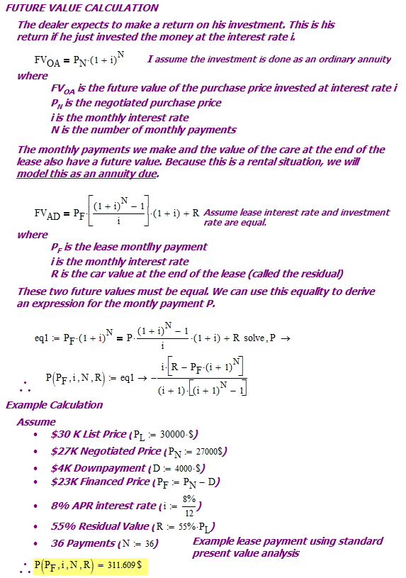
Figure 1 summarizes the derivation of the lease from the future value standpoint. It includes a worked example that shows how to handle the case of making a down payment and negotiating a lower price. As stated earlier, the example is from here. Note that I model the lease payments as an annuity due (information here).

Figure 1: Derivation of Lease Payment Formula From Future Value Standpoint.

Figure 1: Derivation of Lease Payment Formula From Future Value Standpoint.

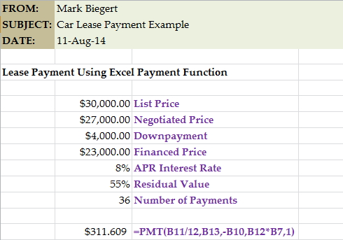
Appendix A shows the same calculation performed using Excel. The results are identical.

Present Value Viewpoint

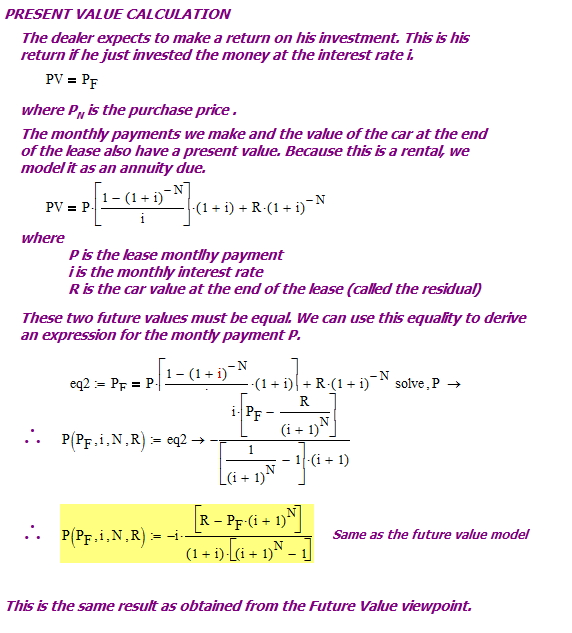
Figure 2 shows how the same lease payment formula can be derived from the present value viewpoint.

Figure 2: Derivation of Lease Payment Formula From Present Value Standpoint.

Figure 2: Derivation of Lease Payment Formula From Present Value Standpoint.

Money Factor Viewpoint

This analysis is interesting to me because of its focus on dealing with averages. Here is a summary of the approach.

  • Cars are a depreciating asset. The person leasing the car must pay the depreciation.
  • The total interest paid on the lease is equal to the total payments made minus the amount financed (PF).
  • The amount of the payment is equal to the average interest paid per payment plus the average depreciation paid per payment.

We can summarize the last bullet with Equation 1.

Eq. 1 P={{P}_{I}}+{{P}_{D}}

where

  • P is the monthly lease payment
  • PI is the average interest paid per lease payment
  • PD is the average amount of depreciation paid off per lease payment

We can calculate the average depreciation paid per payment as shown in Equation 2.

Eq. 2 {{P}_{D}}=\frac{P_F-R}{N}

Determining the average interest paid per payment is a bit more complicated. The keys to determining this relationship are:

  • P=\frac{i\cdot \left( {{P}_{F}}\cdot {{\left( 1+i \right)}^{N}}-R \right)}{{{\left( 1+i \right)}^{N}}-1}
  • Use of the Taylor series substitution {{\left( 1+i \right)}^{N}}\approx 1+N\cdot i+\frac{{{N}^{2}}\cdot {{i}^{2}}}{2}.
  • This means that P\approx \frac{PP\cdot i\cdot \left( 1+N\cdot i+\frac{{{N}^{2}}\cdot {{i}^{2}}}{2} \right)-R\cdot i}{\left( 1+N\cdot i+\frac{{{N}^{2}}\cdot {{i}^{2}}}{2} \right)-1}.

Equation 3 summarizes the derivation.

Eq. 3 {{\left. {{P}_{I}}=\frac{P\cdot N-\left( PP-R \right)}{N} \right|}_{P\approx \frac{PP\cdot i\cdot \left( 1+N\cdot i+\frac{{{N}^{2}}\cdot {{i}^{2}}}{2} \right)-R\cdot i}{\left( 1+N\cdot i+\frac{{{N}^{2}}\cdot {{i}^{2}}}{2} \right)-1}}}
After much painful algebra ...
{{P}_{I}}=\frac{i\cdot \left( P_F+R+N\cdot P_F\cdot i \right)}{N\cdot i+2}
{{P}_{I}}=\frac{\frac{i}{2}\cdot \left( P_F+R \right)+\left( N\cdot i \right)\cdot \frac{i}{2}\cdot P_F}{1+N\cdot \frac{i}{2}}
Assume that P_F+R\gg \left( N\cdot i \right)\cdot P_F, which means that P_F can be replaced by \frac{P_F+R}{2} with minimal error.
{{P}_{I}}\approx \frac{\frac{i}{2}\cdot \left( P_F+R \right)+\left( N\cdot i \right)\cdot \frac{i}{2}\cdot \left( \frac{P_F+R}{2} \right)}{1+N\cdot \frac{i}{2}}
{{P}_{I}}=\left( P_F+R \right)\cdot \frac{i}{2}\cdot \frac{1+N\cdot \frac{i}{2}}{1+N\cdot \frac{i}{2}}
\therefore {{P}_{I}}\approx \left( {{P}_{F}}+R \right)\cdot \frac{i}{2}=\left( {{P}_{F}}+R \right)\cdot \frac{I}{24}

We can substitute Equations 2 and 3 into Equation 1 to obtain Equation 4, which is the equation the auto dealers use.

Eq. 4 P=\frac{P_F-R}{N}+\left( P_F+R \right)\cdot \frac{I}{24}

Figure 3 shows that we can work the example of Figure 1 without using powers of numbers and obtain nearly the same answer with much less mathematical effort.

Figure 3: Worked Example Using Money Factor.

Figure 3: Worked Example Using Money Factor.

The exact solution gives a payment value of $311.61 and the approximation gives $312.22. This is an error of 0.2%. Not too shabby.

Conclusion

In this post I looked at leasing from a classical viewpoint (present value and future value) and from an approximate viewpoint (money factor). I worked through an example that show that difference between the results is a fraction of a percent. This approximation makes sense for common use because it avoids the human calculator from needing to deal with powers of numbers, which for many folks is an issue.

Appendix A: Car Lease Payment Calculation in Excel

Figure 4 show the same calculation done using the Excel PMT function.

Figure 4: Lease Payment Calculation Using Excel.

Figure 4: Lease Payment Calculation Using Excel.

Posted in Financial | 12 Comments

Projectile Time of Flight/Distance Versus Velocity

Introduction

As I mentioned before, I am reading the book "Modern Practical Ballistics" by Pejsa and am finding some interesting material there. I previously duplicated Peja's derivation for a function describing a G7 standard projectile's velocity versus range. This post will briefly look at functions for time of flight and range. I recommend going straight to the Pejsa book for those wanting a deeper dive into the subject. Note that Pejsa strictly uses imperial units. I will continue to use those units here, but the Mathcad routines shown are setup so that they will work with metric units as well.

While this derivation is centered on the G7 standard projectile, the results can be applied to a general projectile through the use of the ballistic coefficient. I will go through the details of this adjustment in a later post.

Analysis

Background

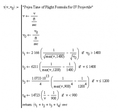
In my previous post, I only addressed velocities above 1400 feet per second (fps) to keep the functions simple. Pejsa actually addresses velocities all the way down to zero. After thinking about it, I decided it would be useful to show how one could express a complicated function in a computer algebra system, like Mathcad. Figure 1 shows the function that Pejsa uses for the entire range of velocities. This function is based on polynomials fit the G7 drag data.

Eq. 1

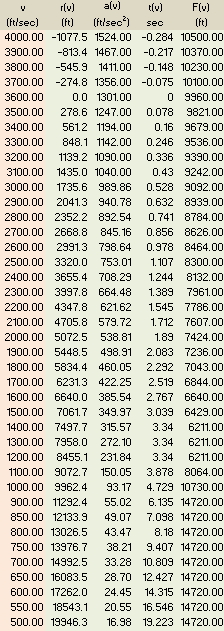
This function is represented by a Mathcad program. Using this acceleration function, I have generated a table of acceleration values versus some velocity values. This same table of data is in the Pejsa book.

Derivation of Time of Flight Formula

As discussed in a previous post, the acceleration of a projectile is modeled by Equation 2. Note that the exponent is modeled by 2 - n. This has to do with the drag coefficient being defined with respect to v2.

Eq. 2 a(v)=\frac{dv}{dt}=-k\cdot {{v}^{2-n}}
\frac{dv}{{{v}^{2-n}}}=-k\cdot dt\Rightarrow {{v}^{n-2}}\cdot dv=-k\cdot dt
\int\limits_{{{v}_{0}}}^{v}{{{v}^{n-2}}\cdot dv}=\int\limits_{0}^{t}{-k\cdot dt}
\left. \frac{{{v}^{n-1}}}{n-1} \right|_{{{v}_{0}}}^{v}=-k\cdot t
\frac{{{v}^{n-1}}-v_{0}^{n-1}}{n-1}=-k\cdot t
\therefore t=\frac{{{v}^{n-1}}-v_{0}^{n-1}}{k\cdot \left( n-1 \right)}

The value of the exponent correction n varies with velocity range as shown in Table 1.

Table 1: Drag Equation Exponent Corrections.
Velocity Range n
(exp correction)
0 fps < v ≤ 900 fps 0.0
900 fps < v ≤ 1200 fps -3.0
1200 fps< v ≤ 1400 fps 0.0
v > 1400 fps 0.5

Using Equation 2 and Table 1, we can derive a function for the time of flight (Equation 3).

Eq. 3

Distance Versus Velocity

A similar analysis can be done to obtain a distance versus velocity equation and table of data. Equation 4 shows the derivation.

Eq. 4 a(v)=\frac{dv}{dt}=-k\cdot {{v}^{2-n}}
\frac{dv}{dx}\cdot \frac{dx}{dt}=-k\cdot {{v}^{2-n}}
\frac{dv}{dx}\cdot v=-k\cdot {{v}^{2-n}}
\frac{dv}{dx}=-k\cdot {{v}^{1-n}}
\int\limits_{{{v}_{0}}}^{v}{{{v}^{n-1}}\cdot dv}=\int\limits_{0}^{x}{-k\cdot dx}
\left. \frac{{{v}^{n}}}{n} \right|_{{{v}_{0}}}^{v}=\frac{1}{n}\cdot \left( {{v}^{n}}-v_{^{0}}^{n} \right)=-k\cdot x
\therefore x=\frac{1}{n \cdot k} \cdot \left( v_{^{0}}^{n}-{{v}^{n}} \right)

Equation 5 and Table 1 allows us to generate the corresponding Mathcad program and output results. These results duplicate the results from Pejsa for a G7 projectile.

Eq. 5

Conclusion

Figure 1 summarizes all the data generated above, plus adds the data for F. The exact same table is at the back of Pejsa Chapter 8. Notice how I used an Excel component to allow me to format the table.

Figure 1: Generated Full G7 Data Table.

Figure 1: Generated Full G7 Data Table.

Posted in Ballistics | 5 Comments

Drive-By Math

Quote of the Day

It is failure that guides evolution; perfection provides no incentive for improvement, and nothing is perfect.

— Colson Whitehead


Introduction

Figure 1: Illustration of Level Translation.

Figure 1: Illustration of Level Translation.

Occasionally, I have an engineer come by my cube and unexpectedly present me with an opportunity to do math. A few years ago one of the engineers stopped by with a VERY common type of electrical engineering problem. He had an LVPECL logic device that needed to connect to a CML logic device. Of course, these two logic families have different voltage levels and cannot communicate with one another unless some sort of voltage-level shifting (Figure 1) is performed between the devices. We had been using a level-shifting circuit recommended by an IC vendor, but that circuit had turned out to have some problems (I do not know what these problems were). The engineer posing the question had spent a few hours grinding through the math manually and eventually decided that it was too painful to continue. He knew that I use computer algebra systems like Mathematica and Mathcad, so he asked if I could help. Using Mathcad, the following analysis was performed and we had a solution within five minutes. It was quite a demonstration of the power of modern computer algebra systems.

Analysis

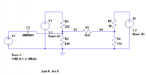
Figure 2 shows the circuit that I was presented with.

Figure 1: Schematic of the Level Matching Network Under Consideration.

Figure 2: Schematic of the Level Matching Network Under Consideration.

From my standpoint, I knew nothing about his problem. I treated this purely as a circuit analysis problem. The engineer told me that this circuit had to meet a number of constraints.

  • V1 = 3.3 V (a supply voltage)
  • V2 = 1.3 V (another supply voltage)
  • V3 = 1.3 V (see schematic)
  • V4 = 1.1 V (see schematic)
  • Zn3 = 50 Ω (input impedance at V3)
  • Reduce the signal level by 1/2 at V4

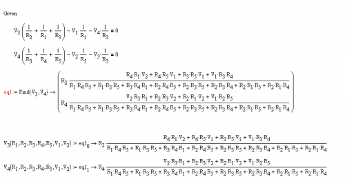
I began by writing Kirchoff''s equations for this circuit in Mathcad and solving for the voltages V3 and V4. Figure 3 illustrates this calculation. This result took me a couple of minutes in Mathcad. The engineer who posed the question had worked hours on it.

Figure 2: Nodal Equations and Solution for Figure 1 Schematic.

Figure 3: Nodal Equations and Solution for Figure 1 Schematic.

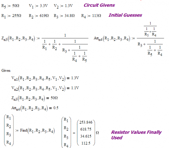
Now that I had my equations for V3 and V4, I can use Mathcad's Solver block to select the resistors required to meet the circuit constraints. Figure 4 shows this calculation.

Figure 3: Resistor Value Determination.

Figure 4: Resistor Value Determination.

This completed the analysis and the engineer went away. I assumed everything went well because the engineer went away with a smile on his face. This effort resulted in a bit of humor a few months later. The worksheet was put together quickly so it is not very neat -- here is the source.

Conclusion

A few months after this exercise, I was taking with some engineers about how a circuit card that previously had problems was now performing very well. They mentioned that a level-shifting circuit had been a problem but that the issue had been resolved. I asked who had resolved the problem and they said I had! I had no clue what I was working on during my little analysis effort. It turned out this level shifting circuit had been a problem, and my new resistor values had been incorporated – they worked as expected.

This circuit has now been in production for a number of years. When people ask about whether computer algebra systems are useful to engineers, I always use this circuit as my best example.

Save

Save

Save

Save

Posted in Electronics | 3 Comments

Calculating the Density of a Planet

Quote of the Day

Democracy is the theory that the common people know what they want, and deserve to get it good and hard.

H. L. Mencken


Introduction

Figure 1: Artist's impression_dwarf_planet_Eris

Figure 1: Artist's Impression of the dwarf planet
Eris. (Source)

I have been reading some interviews with Michel Brown, an astronomer that has a book out called "How I Killed Pluto and Why It Had it Coming." His interviews are interesting and I encourage people to read or view them (Example). Michael is the discoverer of the Kuiper Belt object ("dwarf planet") called Eris and its moon Dysnomia (Figure 1). I became intrigued during one of these interviews when it was mentioned that if a moon is found around a planet, we can compute the planet's density. Let's look at Mike's planet Eris and its moon Dysmonia and see if we can compute the density of Eris.

Analysis

You can use Newton's law of gravity, the equation for centripetal acceleration, and the definition of density to determine the density of a planet. I like to use a computer algebra system to experiment with a problem. For this demonstration, I will use the symbolic solver in Mathcad to help me out. All of the data I used in my analysis came from the Wikipedia. The analysis itself is shown in Figure 1.

Figure 1: Determination of a Planet's Density from Satellite Data.

Figure 1: Determination of a Planet's Density from Satellite Data.

Conclusion

According to my calculations, Eris's density is almost 2.5 gm/cm3. This is in the density range listed in the Wikipedia for Eris. This is a good example of a basic astronomical calculation that can help researchers determine the characteristics of worlds that we can only see as distant objects.

Save

Posted in Astronomy | 1 Comment

Neat Use of Gravity Measurements

Quote of the Day

Your time is limited, so don't waste it living someone else's life.

— Steve Jobs


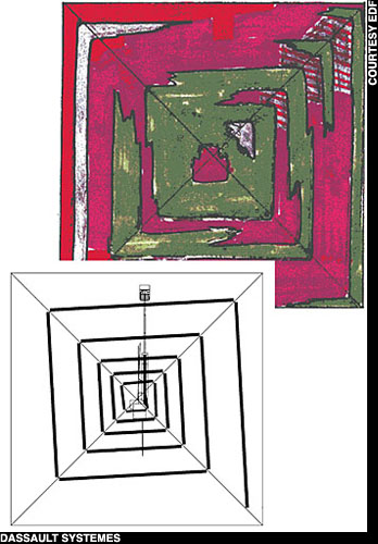
One of my sons is into archeology. Whenever he talks about it, I always find the discussion interesting. We were talking about the pyramids one day and the subject of the various ramp theories came up. He pointed me to an article in Archeology Magazine. Scientists had used a very sensitive new instrument for measuring the gravity field around the pyramid. Here is a graphic of the gravity field.

Figure 1: Gravity Field around the Great Pyramid.

Figure 1: Gravity Field around the Great Pyramid.

After all these thousands of years, it is almost like you see the ramp wrapping around the pyramid in this graphic. Remarkable. Even after all these thousands of years, the ramp's effect on the gravity field of the pyramid is still there.

Posted in History of Science and Technology | Tagged , | Comments Off on Neat Use of Gravity Measurements

An Analog Circuit Design Review

Quote of the Day

The gods do not deduct from a man's allotted span the hours spent in fishing.

— Babylonian Proverb


Introduction

When an electrical engineer asks me what my specialty is, I always respond that I am an analog designer. I love designing analog electronics. Even though I am now in management and am not allowed to design analog electronics professionally anymore, I still design analog electronics in my spare time. As with all professions, analog design has its superstars. When I think about who the analog design superstars are, three names come to mind.

Everything these folks publish should be closely studied by all analog designers. I thought I would spend a little time going over one Woodward's designs. There is an elegance to his work that I find very interesting and his designs always draw me in.

Analysis

This post is review of an article in Electronics Design. I do not want to bore the general audience with the little details that analog people like to dwell on. In this post, I will simply walk through the high-level details. This will give people a little feel for the kind of analysis that occurs in these circuits.

High-Level View

The basic application is an analog circuit that can determine the temperature of a remote sensor. The application block diagram view is shown in Figure 1.

Figure 1: Basic Application Block Diagram.

Figure 1: Basic Application Block Diagram.

The basic requirements of this application are:

  • Temperature must be measured with an accuracy of ±1°C.
  • The sensor is driven over "long wires," which means the wires have enough resistance that the resistance cannot be neglected.
  • Absolute minimum cost is critical – we do not want to spend money on processors, memory, and software.
  • We want a circuit that requires simple or no calibration.
  • The output of the circuit must be a voltage in the range 0 V to 10 V that is directly proportional to the temperature of the sensor over a range of temperatures from 0 °C to 100 °C.

Approach

Woodward's approach is an extension of a design by Jim Williams. The key features of the Woodward design are:

  • Use an inexpensive Bipolar Junction Transistor (BJT) as a the sensor.
    BJTs like the 2N2222 are cheap and the variation of a BJT's base-emitter voltage (VBE) is very predictable with temperature
  • Take VBE readings at three different current levels.
    As will be shown below, measuring VBE at two current levels allows variations in transistor characteristics to be eliminated. Woodward adds a third current level to the algorithm, which can be used to eliminate the voltage variation due to wire losses.
  • Use a very clever multiplexer and difference amplifier circuit to output a voltage proportional to temperature.
    Woodward stores the sensor readings that he makes on capacitors that are switched in at times that allow him to subtract the voltage reading from one another. As is shown below, this subtraction is critical to removing all component and wire loss variations.

The Sensor

Inexpensive Bipolar Junction Transistors (BJTs) that make excellent temperature sensors that cost pennies in volume. Bob Pease does a wonderful job going through the details of using a BJT as a temperature sensor. Equation 1 summarizes the nuances in this excellent article.

Eq. 1 {{V}_{BE}}=\frac{k_B \cdot T}{q} \cdot \ln \left( \frac{{{I}_{BE}}}{{{I}_{S}}} \right)

where

  • IS is the saturation current of the base-emitter junction. It varies with each transistor.
  • kB is Boltzman's constant.
  • T is the temperature in Kelvin.
  • VBE is the transistor's base-emitter voltage.
  • IBE is the base-emitter current through the transistor.

Except for T, all the parameters in Equation 1 are constants. This means that Equation 1 varies linearly with temperature. Unfortunately, IS is a constant that varies with each transistor. Jim Williams has shown that you can eliminate the variation with IS by taking VBE readings at two current levels and subtracting the results. I duplicate his work in Equation 2.

Eq. 2 {{V}_{BE1}}=\frac{{{k}_{b}}\cdot T}{q}\cdot \ln \left( \frac{{{I}_{BE1}}}{{{I}_{S}}} \right),{{V}_{BE2}}={{\frac{{{k}_{b}}\cdot T}{q}}}\cdot \ln \left( \frac{{{I}_{BE2}}}{{{I}_{S}}} \right)
and \Delta {{V}_{BE}}={{V}_{BE1}}-{{V}_{BE2}}=\frac{{{k}_{b}}\cdot T}{q}\cdot \ln \left( \frac{{{I}_{BE1}}}{{{I}_{BE2}}} \right)

where VBE1 is the base-emitter voltage at IBE1 and VBE2 is the base-emitter voltage at IBE2. In Equation 2, ΔVBE has a linear temperature variation and all the other parameters are not subject to component variations.

Equation 2 shows us that simply subtracting the VBE values at two different current levels will give us a value that varies directly with absolute temperature (°K). But we cannot measure VBE directly because we have losses in the wire. How do we deal with those?

Wire Losses

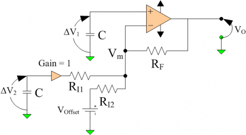
Figure 2 shows the the model I will use for analyzing how Woodward drives the sensor. Note that I have lumped all the wire resistance into a single variable RLoss.

Figure 2: Wire and Sensor Model.

Figure 2: Wire and Sensor Model.

In Equation 3, I define two variables, ΔV1 and ΔV2. ΔV1 is the difference in VLine when the stimulus is IBE = IBE2 +IBE1 and IBE = IBE1. Similarly, ΔV2 is the difference in VLine when the stimulus is IBE = IBE3 +IBE1 and IBE = IBE1. Woodward also sets IBE3=2IBE2. Woodward uses an operational amplifier hooked up as a differential amplifier to create an output voltage equal to 2ΔV1 -ΔV2. As is shown in Equation 3, this linear combination eliminates the terms due to wire loss! We now have an output voltage that varies linearly with absolute temperature (°K).

Eq. 3 \Delta {{V}_{1}}=\frac{{{k}_{b}}\cdot T}{q}\cdot \ln \left( \frac{{{I}_{BE2}}+{{I}_{BE1}}}{{{I}_{BE1}}} \right)+{{I}_{BE2}}\cdot {{R}_{W}}
\Delta{{V}_{2}}=\frac{{{k}_{b}}\cdot T}{q}\cdot \ln \left( \frac{{{I}_{BE3}}+{{I}_{BE1}}}{{{I}_{BE1}}} \right)+{{I}_{BE3}}\cdot {{R}_{W}}
\Delta{{V}_{2}}=\frac{{{k}_{b}}\cdot T}{q}\cdot \ln \left( \frac{2\cdot {{I}_{BE2}}+{{I}_{BE1}}}{{{I}_{BE1}}} \right)+2\cdot {{I}_{BE2}}\cdot {{R}_{W}}
\Delta {{V}_{1}}-\Delta {{V}_{2}}=\frac{{{k}_{b}}\cdot T}{q}\cdot \ln \left( \frac{{{\left( {{I}_{BE2}}+{{I}_{BE1}} \right)}^{2}}}{{{I}_{BE1}}\cdot \left( {{I}_{BE3}}+{{I}_{BE1}} \right)} \right)

Unfortunately, Equation 3 has a non-zero value at 0 °C because T is expressed in absolute temperature (°K). We now need to make this output voltage vary linearly with Celsius temperature (°C).

Linear Variation with °C

The final bit of analog signal processing is fairly straightforward. We have three things to do:

  • Generate the linear combination 2ΔV1(T) -ΔV2(T).
    This computation eliminates voltage loss other than from the transistor BE junction.
  • Shift this curve down by the value of 2ΔV1(273.15 °K) -ΔV2(273.15 °K).
    273.15 °K is the same as 0 °C. This makes our output voltage equal to 0 V when T = 0 °C.
  • Apply gain to the circuit to scale the output so that 0 °C to 100 °C is represented by 0 V to 10 V.
    The voltage range of 0 V to 10 V is arbitrary, but is easy to measure accurately. Figure 3 shows a simplified version of Woodward's output circuit.
Figure 3: Output Amplifier Circuit.

Figure 3: Output Amplifier Circuit.

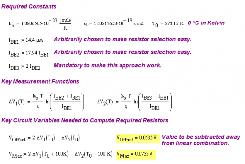
We need to compute some resistor values for this circuit. I will use Mathcad for this part of the exercise. First let's define some terms and functions (Figure 4).

Figure 4: Definitions for Computational Work.

Figure 4: Definitions for Computational Work.

We now need to derive an expression for the output voltage from the op-amp in terms of resistors (Figure 5). Note that some expression were long and are chopped in Figure 5. That happens sometimes.

Figure 5: Solve for the Op-Amp Output Voltage.

Figure 5: Solve for the Op-Amp Output Voltage.

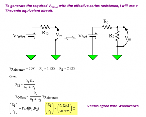
These resistor values work for the circuit of Figure 3, but VOffset is a small value that is difficult to generate directly. Woodward used a Thevenin equivalent circuit to generate the offset voltage and required input resistance. I compute these values in Figure 6.

Figure 6: Thevenin Equivalent Circuit for Generating the Offset Voltage.

Figure 6: Thevenin Equivalent Circuit for Generating the Offset Voltage.

All resistances are now determined. The capacitor values are not particularly critical and I will not go into detail as to how they are selected.

Circuit Sequencing

The circuit is a bit confusing until you see that it uses a two-bit counter to cycle through the stimulus current values (see Figure 7). This counter applies currents to the transistor sensor in the order I1, I1+I2, I1, I1+I3. If you look at the circuit carefully, you will see that Woodward is using the multiplexer to charge the 1 μF capacitors with the proper polarities so that their sums generate ΔV1 and ΔV2. It is a little tricky, but just look at Figure 7 carefully and you will see how he does it.

Schematic

I have included the schematic for reference in Figure 7 (Source).

Figure 7: Woodward Schematic.

Figure 7: Woodward Schematic.

Conclusion

This circuit is very representative of Woodward's work. His circuits are fine examples of applying component physics in an economical fashion to real-world applications. I will have a few more posts that cover some of his other work.

Posted in Electronics | Comments Off on An Analog Circuit Design Review

Railroad Math

Introduction

I was listening to an advertisement where CSX made the claim that they move 1 ton of freight 423 miles for 1 gallon of fuel. This is an interesting measure of efficiency. Let's see if we can confirm this using a couple of different analysis approaches.

Top-Down Approach

CSX issues quarterly reports, which contains data that we can use to estimate the miles per gallon-ton of freight. This forum article has some interesting data from the 4Q2007 CSX financial statement.

  • CSX moved 253 billion revenue ton-miles of goods in the 12 months ending 12/31/07.
  • During this period, CSX consumed 569 million gallons of diesel #2 fuel.

This makes computing the efficiency eff of a train (mile-ton per gallon) easy, which is shown in Equation 1.

Eq. 1 \mathit{eff}=\frac{253\text{E9}\cdot \text{mile}\cdot \text{ton}}{569\text{E9}\cdot \text{gal}}=445\frac{\text{mile}\cdot \text{ton}}{\text{gal}}

This number is close to what CSX is using its advertisement. So their number is credible based on their business statment.

Bottom-Up Approach

It is a bit more difficult to look at the problem from the standpoint of friction and energy, but let's take a wack at it.

First, let's gather some data.

  • Energy per gallon of #2 diesel fuel is 138,700 BTU/US gal (Source)
  • Efficiency of a diesel engine is ~46% (Source and Source)
  • Diesel to rail conversion efficiency of 80% (Source)
    There is some loss of power due to transmission inefficiency in the diesel-electrical-rail transfer of power. I am using the value of 80% for the transmission efficiency based on a reference from the 1950s that was comparing steam to diesel-electric locomotives. This number is probably out of date, but is a reasonable start for a rough estimate.
  • Train expends 20 lb of pulling force per ton of load (Source)
    This number is subject to variation due to track condition, weather, grade, and curvature of the track. I am assuming an average value that is in the ballpark, but could easily be off by ±20% or more. Remember, we are just trying to determine if the CSX efficiency number is reasonable.

I would propose that one simple model would be to equate the energy dissipated against the rolling resistance of the train to the energy available from a gallon of diesel fuel.

Eq. 2 {{F}_{FrictionPerTon}}\cdot d={{E}_{FuelOilPerGal}}\cdot {{e}_{Diesel}} \cdot e_{c}

Where d is the distance traveled, FFrictionPerTon is the resistance of a ton of load (= 20 lb per ton), EFuelOilPerGal is the energy per gallon of #2 diesel fuel (=138,700 BTU/US gal), eDiesel is the efficiency of a modern diesel engine (=46%), and ec is the diesel-to-rail conversion efficiency (=80%).

We can solve Equation 2 for d and substitute our assumed values.

Eq. 3 d=\frac{{{E}_{FuelOilPerGal}}\cdot {{e}_{Diesel}} \cdot e_c }{{{F}_{FrictionPerTon}}}=376\frac{\text{mile}\cdot \text{ton}}{\text{gal}}

This value is close enough that feel I have verified the CSX number from the bottom up.

Conclusion

Moving one ton of freight 423 miles on one gallon of fuel seems like a reasonable value. This exercise really shows the efficiency of moving material in bulk.

Posted in General Science | 5 Comments

Drinking Math

Quote of the Day

The difficulty lies not so much in developing new ideas as in escaping from old ones.

- John Maynard Keynes


Introduction

Figure 1: I used to love to see people make layered drinks.

Figure 1: As a boy, I used to love to see people make layered drinks. The first layered drink I saw as a boy was a zombie. (Source)

As a non-drinker, I have never had much interest in alcohol. That said, alcohol has been a big part of my life. My mother earned her living working in bars, starting as a waitress and eventually managing them. Even in retirement, she works part-time selling pull tabs in bars for local sports groups. I have also been the designated driver for literally hundreds of social occasions. At work, I have had numerous co-workers who have derived much pleasure brewing beer and wine. As a boy, I did find the layered drinks interesting (e.g. Figure 1), but only because they looked cool.

But alcohol must be used in moderation. To help guide people in their consumption, there are numerous charts and tables that tell people how much they can drink and remain under the legal limits. While prowling around the Wolfram Alpha web site, I noticed that they have a Blood Alcohol Content (BAC) calculator. I started looking at the output and I saw that there was some interesting math going on there.

For those who are interested, I have implemented the formulas below in an Excel spreadsheet here. Let's dig ...

Analysis

BAC Definition

The Wikipedia provides a very complete definition of BAC and I will start there with a slight paraphrasing of their definition.

BAC is the concentration of alcohol in a person's blood. It is most commonly used as a metric of intoxication for legal or medical purposes. It is usually expressed as a fractional percentage in terms of volume of alcohol per liter of blood in the body.

So BAC is unitless quantity because it is the ratio of two volumes. This definition of BAC is not universal. For example, California actually uses grams (gm) of alcohol per deciliter (100 mL = dL) of blood. For this post, we will use the more common ratio of volumes, which is expressed mathematically in Equation 1.

Eq. 1 BAC\triangleq \frac{{{V}_{Ethanol}}}{{{V}_{Blood}}}

Key Analysis Assumptions

The analysis assumptions in the creation of the BAC tables vary because a person's response to alcohol varies by person. Here are the assumptions that I could identify.

  • The alcohol evenly spreads through all the water of the body, not just the blood.
  • The amount of water in the body is proportional to body weight.
    This assumption is highly variable between individuals. Quoting from the Wikipedia, "In a newborn infant, this may be as high as 75 percent of the body weight, but it progressively decreases from birth to old age, most of the decrease occurring during the first 10 years of life. Gender also affects the percentage of water for an individual. This is because women, on average, have a higher body fat percentage. Higher body fat percentage correlates with lower body water percentages. As such, obesity decreases the percentage of water in the body, sometimes to as low as 45 percent."
  • Every drink has the same amount of alcohol.
    In fact, the amount of alcohol varies by drink. To simplify the discussion, most tables assume a drink contains about 0.5 oz of alcohol by weight. Wolfram Alpha assumes 0.533 gm per drink. Since ethyl alcohol (ethanol) has a density of 0.789 g/cm3, 0.533 oz (mass) of alcohol is equivalent to 0.648 fluid ounces. This amount of alcohol corresponds roughly to the following common drinks:

    • 12 fluid ounces of beer
    • 1.25 fluid ounces of 100 proof liquor
    • 4 fluid ounces of 25 proof table wine
  • The body eliminates alcohol at a fixed rate.
    Quoting the Wikipedia, "The rate of elimination in the average person is commonly estimated at .015 to .020 gm/dL per hour, although again this can vary from person to person and in a given person from one moment to another." To convert the units from gm/(dL hr) to the BAC's unitless over volume/volume, we need to apply the density of ethanol as follows: \left( 0.015-0.020 \right)\cdot \frac{\text{gm}}{\text{dL}\cdot \text{hr}}\cdot \frac{\text{c}{{\text{m}}^{3}}}{\text{0}\text{.789}\cdot \text{gm}} = \left( 0.19\%-0.25\% \right)\frac{1}{\text{hr}}.

Modeling BAC

Everything I have been able to find on the web uses the model shown in Equation 2 with different parameters.

Eq. 2 BAC=\frac{n\cdot \gamma }{\frac{w\cdot \alpha }{{{\rho }_{{{H}_{2}}O}}}}-\beta \cdot t

where

  • w is the weight in pounds
  • n is the number of drinks
  • t is the time since consumption (hours)
  • ? is the percentage of water in a body (weight of water/body weight = ~75%)
  • ? is volume of ethanol in a drink (0.648 fluid ounces)
  • ? is the rate of elimination (~0.021% per hour)
  • ?H20 is the density of water (1 gm/cm3 = 0.065198 lb/fluid ounce)

If we substitute the values shown into Equation 2 we get Equation 3.

Eq. 3 BAC = 5.633\text{\%} \cdot \frac{n}{w}-0.021\text{\%} \cdot t

Figure 2 shows the Wolfram Alpha result and Figure 3 shows Equation 3 graphed in Mathcad. The results appear identical.

Figure 1: BAC Versus Time for 240 lb Man After 6 Drinks.

Figure 2: BAC Versus Time for 240 lb Man After 6 Drinks.

Figure 2: BAC Model in Mathcad.

Figure 3: BAC Model in Mathcad.

Conclusion

I have looked at a number of web sites on BAC levels and they all make different assumptions about their definition of a drink, body water percentages, and elimination rate. The variation in the assumptions all reflects the fact that these characteristics vary by individual. Other important factors, like how long you were drinking and whether you were consuming food while drinking, are completely ignored. Looks to me like it is difficult to know how many drinks you can have and still drive. Sounds like not drinking and driving is still the best way to go. It's always wise to remember to book another method of transport home after you've been drinking, it's not worth risking lives for. Because, let's face it, most people who do drink and drive end up getting caught one way or another and will end up looking to get useful information from a criminal defense attorney in anticipation of charges being brought against them. Drunk driving is one of the top causes of car accidents, which is why it's important to avoid driving a vehicle after drinking alcohol. Unfortunately, most drunk drivers end up needing personal injury attorneys to support them after they have put themselves, and other road users, in danger. To prevent yourself from injuring anyone, consider booking a taxi after any social events, or ask family and friends if they can collect you.

Posted in Health | 9 Comments

Interesting Old Submarine Photo

A co-worker and I were discussing strange photos we have seen. I mentioned a photo that I saw years ago that showed USS S-5's tail sticking out of the water. During the 1920s, submarines that submerged occasionally did not come back up. In this case, the crew was very clever. The submarine was 231 feet long and sank in 194 feet of water. The crew was able to lighten the aft section and float the tail of the sub up to the surface. With great difficulty, they cut a hole in the tail and waited for a ship to come by. No one lost their life, which for early submarines is an amazing statement. Figure 1 shows the tail section protruding from the water. I cannot imagine how difficult it must have been for the crew to move around in a small sub with its end tipped up. Also, the aft area necks down to become pretty tiny. It must have been extremely cramped.

Figure 1: USS S5 Tail Protruding Above the Water.

Figure 1: USS S5 Tail Protruding Above the Water.


If you would like to read more about the S-5 and its sinking, see this web site. A book has been written about the incident called "Under Pressure: The Final Voyage of Submarine S-Five" by A.J. Hill.

Here is another photograph showing a rescue ship.

Figure 2: S-5's Tail Near One of Its Rescuers.

Figure 2: S-5's Tail Near One of Its Rescuers.

Posted in History of Science and Technology | Tagged | Comments Off on Interesting Old Submarine Photo

"Dying Gasp" from a Circuit Standpoint

Introduction

The Metro Ethernet Forum (MEF) specifies requirements for carrier-grade Ethernet services. One the features they define is the "dying gasp". A dying gasp is defined as follows:

Dying Gasp is a message (or signal) sent by the Customer Premises Equipment (CPE) to the service provider when a power outage occurs.

In most cases, the hardware does not know that the power is failing until the power is already starting to go away. The dying gasp protocol requires that three "I am dying" messages be sent before the CPE gear goes down for good, which means the CPE must stay operating for about 3 msec after the power has gone away. To accomplish this feat, we need to include some local energy storage with MEF-compliant Ethernet hardware. This post will examine how we can estimate the amount of local energy storage required.

Analysis

We will begin by assuming the power supply architecture shown in Figure 1.

Figure 1: Circuit Model for "Dying Gasp" Capacitive Backup.

Figure 1: Circuit Model for "Dying Gasp" Capacitive Backup.

There are a few points that should be made about this power supply architecture:

  • The input circuit will only conduct current one way.
    We need to make sure that as the power drops away, the power we need for our Ethernet interface is not drawn out of the input. In Figure 1, I show a diode, but there are number of ways of isolating the backup capacitor from the dying power source. In most cases, FETs would be more efficient than diodes, but diodes are simpler to understand. However, all this is an implementation detail.
  • The load requirements are modeled as a current source.
    In most cases, we are trying to provide backup energy for a switching power supply, which draw relatively constant power over a range of voltages.
  • Energy is stored in capacitors.
    In most cases, capacitors are the cheapest and easiest way of storing backup energy. This assumes the required backup time is small (~msec). As times get longer, batteries look better.

Energy-Based Capacitance Requirement Determination

If first worked the problem from an energy standpoint. Recall from basic physics that energy stored on a capacitor is given by Equation 1.

Eq. 1 {{E}_{Capacitor}}=\frac{1}{2}\cdot {{C}_{Backup}}\cdot V_{Capacitor}^{2}

The energy needed to power our MEF-compliant device is given by Equation 2.

Eq. 2 {{E}_{Total}}=P\cdot {{T}_{DyingGasp}}=\frac{1}{2}\cdot {{C}_{Backup}}\cdot \left( V_{Initial}^{2}-V_{Final}^{2} \right)

where

  • P is the power draw of our MEF-compliant device.
  • TDyingGasp is the time required to transfer the three dying gasp messages.
  • VInitial is the initial voltage on the backup capacitor. This is the voltage on the backup capacitor at the moment power drops away.
  • VFinal is the final voltage on the backup capacitor and is the minimum voltage at which load input can function.
  • CBackup is the capacitance of the backup capacitor.

We can use Equation 2 to solve for CBackup (Equation 3).

Eq. 3 \therefore {{C}_{Backup}}=\frac{2\cdot P\cdot {{T}_{DyingGasp}}}{V_{Initial}^{2}-V_{Final}^{2}}

Current-Based Capacitance Requirement Determination

The backup capacitance requirement is given by Equation 3, but some electrical engineers do not like energy-based arguments. They prefer arguments based on circuit parameters like voltage and current, which can be measured directly. We can obtain the same result using circuit parameters as follows.

The current drawn by the load and the current drawn from the capacitor are given by Equation 4.

Eq. 4 {{I}_{Load}}=\frac{{{P}_{Load}}}{{{V}_{Load}}}={{C}_{Backup}}\cdot \frac{d{{V}_{Load}}}{dt}

Equation 5 shows Equation 4 broken up into its differential form.

Eq. 5 {{V}_{Load}}\cdot d{{V}_{Load}}=\frac{{{P}_{Load}}}{{{C}_{Backup}}}\cdot dt

We know can integrate both sides of Equation 5, as is illustrated in Equation 6.

Eq. 6 \int\limits_{{{V}_{Initial}}}^{{{V}_{Final}}}{{{V}_{Load}}\cdot d{{V}_{Load}}}=\int\limits_{0}^{T}{\frac{{{P}_{Load}}}{{{C}_{Backup}}}\cdot dt}
\left. \frac{V_{Load}^{2}}{2} \right|_{{{V}_{Initial}}}^{{{V}_{Final}}}=\frac{V_{Initial}^{2}-V_{Final}^{2}}{2}=\frac{{{P}_{Load}}}{{{C}_{Backup}}}\cdot T
\therefore {{C}_{Backup}}=\frac{2\cdot P\cdot {{T}_{DyingGasp}}}{V_{Initial}^{2}-V_{Final}^{2}}

As we would expect, both methods yield the same result.

Empirical Example

I threw the calculations into Mathcad and put the screenshot into Figure 1.

Figure 1: Calculation Used for Actual Product.

Figure 1: Calculation Used for Actual Product.

Conclusion

One of the more difficult parts of product development is determining requirements, a process I call "The Treasure Hunt." The analysis shown here describes a very common type of analysis that is done to determine capacitor requirements for backup systems.

Posted in Electronics | Tagged , , | 6 Comments