
Introduction
I was listening to an advertisement where CSX made the claim that they move 1 ton of freight 423 miles for 1 gallon of fuel. This is an interesting measure of efficiency. Let's see if we can confirm this using a couple of different analysis approaches.
Top-Down Approach
CSX issues quarterly reports, which contains data that we can use to estimate the miles per gallon-ton of freight. This forum article has some interesting data from the 4Q2007 CSX financial statement.
- CSX moved 253 billion revenue ton-miles of goods in the 12 months ending 12/31/07.
- During this period, CSX consumed 569 million gallons of diesel #2 fuel.
This makes computing the efficiency eff of a train (mile-ton per gallon) easy, which is shown in Equation 1.
| Eq. 1 |  |
This number is close to what CSX is using its advertisement. So their number is credible based on their business statment.
Bottom-Up Approach
It is a bit more difficult to look at the problem from the standpoint of friction and energy, but let's take a wack at it.
First, let's gather some data.
- Energy per gallon of #2 diesel fuel is 138,700 BTU/US gal (Source)
- Efficiency of a diesel engine is ~46% (Source and Source)
- Diesel to rail conversion efficiency of 80% (Source)
There is some loss of power due to transmission inefficiency in the diesel-electrical-rail transfer of power. I am using the value of 80% for the transmission efficiency based on a reference from the 1950s that was comparing steam to diesel-electric locomotives. This number is probably out of date, but is a reasonable start for a rough estimate. - Train expends 20 lb of pulling force per ton of load (Source)
This number is subject to variation due to track condition, weather, grade, and curvature of the track. I am assuming an average value that is in the ballpark, but could easily be off by ±20% or more. Remember, we are just trying to determine if the CSX efficiency number is reasonable.
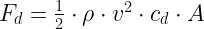
I would propose that one simple model would be to equate the energy dissipated against the rolling resistance of the train to the energy available from a gallon of diesel fuel.
| Eq. 2 |  |
Where d is the distance traveled, FFrictionPerTon is the resistance of a ton of load (= 20 lb per ton), EFuelOilPerGal is the energy per gallon of #2 diesel fuel (=138,700 BTU/US gal), eDiesel is the efficiency of a modern diesel engine (=46%), and ec is the diesel-to-rail conversion efficiency (=80%).
We can solve Equation 2 for d and substitute our assumed values.
| Eq. 3 |  |
This value is close enough that feel I have verified the CSX number from the bottom up.
Conclusion
Moving one ton of freight 423 miles on one gallon of fuel seems like a reasonable value. This exercise really shows the efficiency of moving material in bulk.


 for a G7 Standard Projectile.")
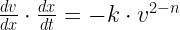
 , where kd and n are projectile-specific constants.
.")


 ).
).


 and
and 


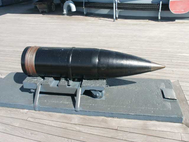
 16-inch Shells.")
, 16 inch Shell (Rotated Horizontal Photo)")


.")


.")


 )
) )
)


 =>
=>  . The equivalence between the other criteria can be demonstrated similarly.