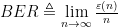
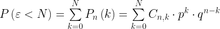
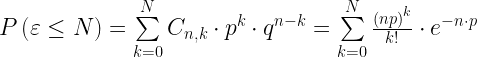
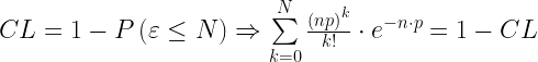
Pope Gregory XIII and Dual Modulus Counters

Quote of the Day

Every new body of discovery is mathematical in form, because there is no other guidance we can have.

— Charles Darwin


Introduction

FIgure 1: Pope Gregory VIII.

Figure 1: Pope Gregory VIII (Source).

I discussed a recent dual-modulus counter design in a previous post. I had not thought much about the history of these counters, but I noticed that our calendar is really a dual-modulus counter. Pope Gregory XIII (Figure 1) established the Gregorian calendar (1582) to resolve issues with the Julian calendar. The reason that calendar development is complicated is because a solar year is 365.24219879 days long, which is not easily expressed in terms of simple integer ratios. Ideally, a calendar system is chosen that is simple and that has a mean year length exactly equal to that of a solar year. While not ideal, the Gregorian calendar provides a simple and fairly accurate approximation to a solar year through the use of a dual-modulus counter design based on years with durations of 365 and 366 days.

Analysis

In the Gregorian calendar, years have lengths of either 365 or 366 days (hence, a dual-modulus). The number of days in a year is given by the following rules

  • Every year that is exactly divisible by four is a leap year, except for years that are exactly divisible by 100.
  • Years exactly divisible by 400 are still leap years.

Using these rules, we can compute the length of a Gregorian year as shown in Equation 1.

Eq. 1 {{T}_{Year}}=\frac{400\cdot 365+3\cdot 24+25}{400}=365.2425\text{ days}

This is a good approximation to the length of a solar year – the error is only 0.0031 days per year. This means that the it will take over 3000 years for the Gregorian calendar to accrue a single day's worth of error.

Save

Posted in Astronomy, Electronics | Tagged , | 1 Comment

The Difficulties Posed By Communications

Quote of the Day

The single biggest problem in communication is the illusion that it's taken place.

- George Bernard Shaw


Figure 1: Time Zones Around the World. (Source)

Figure 1: Time Zones Around the World. (Source)

My company currently has engineering work occurring at a number of sites that are widely separated geographically. For example, much of my time is spent communicating with China and Portugal. Relative to my time zone (Figure 1), China is 14 hours ahead and Portugal is 6 hours ahead.

Trying to coordinate these sites is definitely a challenge. However, this really is nothing new. When I was at HP, my first manager used to say that

Engineering communication reduces by 10 dB per foot.

He used this quote whenever we were trying to move team members physically close to one another to facilitate personal communication. This quote reflected the needs of a time when engineering sites were all in the US and the time zones were within a few hours of one another. It was also a time before email was readily available.

One of my current co-workers made the observation that this quote needs to be updated based on the changes due to new communication technology being implemented into the workplace, like a sip server, amongst others. He said that the statement should be revised to be

Engineering communication reduces by 10 dB per hour of time zone difference.

As I think about it, he is right. Distance does not matter anymore – time does. Working with China means phone calls late at night for someone, and I personally have seen how painful this is. It also means that emails are not answered quickly. Of course, large time zone differences mean that language differences occur, which may be the greatest challenge.

Posted in Management | Tagged , | Comments Off on The Difficulties Posed By Communications

The Law of Employee Retention

I was just interviewing a large number of people as part of an acquisition. After the interviews were done, the interviewers all went out to dinner and discussed the day's events. While at dinner, the topic of employee retention came up. It was during this discussion that I stated my "Law of Employee Retention." The law is simple and is stated in terms of "half-life", which means the time in which 50% of the employees will leave.

An engineer with a spouse whose family is located "far away" has a retention half-life of 5 years.

"Far away" means that the spouse's family is far enough away that plans need to be made to visit them.

I have over 30 years of experience with this rule. I started gathering my data when I was a recruiter with HP. It even worked for me and my wife. I lasted five years with HP before my wife wanted to get closer to her family.

Posted in Management | Tagged , , , | Comments Off on The Law of Employee Retention

Dual Modulus Counter Design Example

Quote of the Day

I have long been of the opinion that if work were such a splendid thing the rich would have kept more of it for themselves.

Bruce Grocott, British politician


Introduction

One of the more common problems in the life of a digital hardware designer is to divide down a master clock to some desired lower frequency value. If life is kind, the master clock is an integer multiple of the desired clock and the problem can be solved with a simple counter. Unfortunately, life is rarely kind and the master clock frequency is usually not an integer multiple of the desired clock. In this case, the designer will need to do a little work. One common solution is to use a dual-modulus counter. This blog will work through an example that came up a while back.

What is a Dual-Modulus Counter?

The dual-modulus counter allows us to design a clock divider with a non-integer modulus, which I call M. Figure 1 illustrates the basic idea. In Figure 1, we desire a modulus that is between N and N-1. We vary the duty cycle of each counter so that the average modulus equals M. Clearly, the instantaneous frequency will never be exactly what we want. But many problems require only that the average value be exactly right and the instantaneous value is of less interest.

Figure 1: Block Diagram of a Dual-Modulus Counter.

Figure 1: Block Diagram of a Dual-Modulus Counter.

Basic Dual-Modulus Mathematics

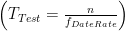
We can compute the modulus we desire using Equation 1.

Eq. 1 M\triangleq \frac{{{f}_{0}}}{{{f}_{D}}}

where M is the desired modulus, f0 is our master clock, and fD is desired output frequency from the dual-modulus divider. Of course, f0 > fD.

Let's assume that N and N-1 are integers such that N > M > N-1. N and N-1 are the moduli of our counter. We can compute the value of N (and correspondingly, N-1) as shown in Equation 2.

Eq. 2 N=\text{ceil}\left( M \right)

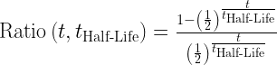
As shown in Equation 3, we can restate M in terms of its integer and fractional part, where the fractional part is assumed to be expressible as an integer ratio A/C.

Eq. 3 M=\left( N-1 \right)+\frac{A}{C}

where A represents the number of N-1 division operations in a cycle and C represents the total number of division cycles (both N and N-1).

Eq. 4 \frac{{{f}_{0}}}{{{f}_{D}}}=\left( N-1 \right)+\frac{A}{C}\Rightarrow \frac{A}{C}=\frac{{{f}_{0}}}{{{f}_{D}}}-(N-1)=\frac{{{f}_{0}}-\left( N-1 \right)\cdot {{f}_{D}}}{{{f}_{D}}}

Ease of implementation requires that we make sure that A and C are relatively prime (i.e. no common factors). Equation 5 shows how to compute both A and C.

Eq. 5 Q=\gcd \left( {{f}_{D}},{{f}_{0}}-\left( N-1 \right)\cdot {{f}_{D}} \right)
A=\frac{{{f}_{0}}-\left( N-1 \right)\cdot {{f}_{D}}}{Q}
C=\frac{{{f}_{D}}}{Q}

Given these equations, we can generate a high-level design for our dual-modulus counter.

One Thing to Note

The dual-modulus counter will divide the master clock by N and N-1. One could do all the divide-by-N operations and then all the divide-by-(N-1) operations. While correct, the generated output clock can have some rather large phase variations from an ideal output frequency. These phase deviations can be minimized by evenly mixing the N and N-1 divisions.

There are various ways to spread the divisions out. I will not dwell on these approaches here, but in the Worked Example below I do illustrate one approach in my Mathcad model.

Worked Example

Computing the Constants

We had a problem a while ago where we needed to generate a 2.048 MHz clock from a 78.125 MHz clock. I threw this example into Mathcad and the results are shown in Figure 2.

Figure 2: Dual-Modulus Worked Example.

Figure 2: Dual-Modulus Worked Example.

Spreading the Different Divisions Out

One can use the modulo operation to spread the different divisions out. Figure 3 illustrates the approach. The vector m in Figure 3 has entries equal to their count values (i.e. 0 to 2047), which means each entry corresponds to a division. I divide by 39 for every entry where the index mod (2048/301) passes through 0 and I divide by 38 for all other entries. The quotient of 2048/301 is the total number of division cycles divided by the number of divide-by-39 cycles. This spreads the divisions out evenly.

Figure 3: Evenly Spreading Out the Divisions.

Figure 3: Evenly Spreading Out the Divisions.

Conclusion

This blog post shows how to design a basic dual-modulus counter. It presents both the theory and a worked example. This example is very similar to a frequency divider that is currently out in the field inside thousands of units.

For an example of a dual modulus counter design that everyone is familiar with, see this post on the Gregorian calendar.

Save

Save

Save

Posted in Electronics | Tagged | 4 Comments

Little Stories from the History of Science and Technology

Introduction

I have always been interested in the connectedness of people. The theory that each of us is separated by only six degrees from anyone else is a theory I like to test. If you examine things carefully, you may find that you have more personal connections to history than you think. I have already written one blog post that alluded to this connectedness. I thought I would write a few more stories.

I am no Wernher Von Braun

Wernher von Braun was one of the great engineers of the 20th century. He clearly was a god to those that worked for him. My story begins when I was working as a contractor on a US Army missile program in the 1990s and was responsible for presenting some work my company was doing. I only had 10 minutes to present, so I simply presented some overview material. After my presentation an old gentleman came up to me and told me that:

"You gave a good presentation, but we are going need much more detail. It would be one thing if you were Wernher von Braun . But you are not Werhner von Braun, at least not yet, and we need much more detail."

While I was a bit shocked, I told the gentleman that next time I would have more detail. Later, I laughed hard about this incident. I found out that the old gentleman had worked under von Braun and held him in total awe. It reminded me of when Lloyd Bentson told Dan Quayle that "You are no Jack Kennedy." Anyway, I now feel like I am two degrees of separation from Wernher von Braun.

My High School Physics Teacher and Wernher von Braun

When I was in high school, my physics teacher (Tom Truax) related a Wernher von Braun story. During the 1960s, there was a huge push to strengthen science and math education in the United States. As part of this effort, Wernher von Braun would occasionally visit teacher conferences around the country. During one conference, he made quite a spectacular arrival. The teachers were all sitting in an auditorium, wondering where their speaker was. Precisely when the speech was scheduled to begin, there was the sound of a helicopter landing on the school grounds. A man in a suit ran out of the helicopter and right onto the podium. He then gave a rousing speech, which concluded by asking "Any questions?" The crowd was silent for a few seconds, so he immediately put his speech away and ran out to the waiting helicopter and flew away. It was quite an impressive display. My physics teacher used to love imitating von Braun's accent in class by saying "Any qvestions?" Anyway, it was the 1960s. Anything could happen.

Earl Bakken, Founder of Medtronic

I spent a summer in 1978 as an engineering intern at Medtronic. It was a large building and one day I got lost. A kindly old man asked me if he could help and I said I was lost. He laughed and asked where I wanted to go. I told him and he guided me to my work area. I thanked him and went about my work. My coworkers were stunned to see me with this gentleman. I asked why and they said, "That is Earl Bakken and he is the founder of Medtronic." Bakken had created largest medical electronics company in the world. All I know was that he was very helpful to a lost young man. While helping me find my way, he also mentioned that he was holding a dancing class and I was welcome to attend. I later found out that he loved to dance and taught classes for people who were interested.

Wozniak and HP

I joined HP in 1979. At one point, I was part of group that was looking at the Apple 2 and trying to determine if there was anything there that HP should be considering in terms of future products. I look back at that effort now and laugh. There were all these stories about Wozniak (who I have never met) trying to convince HP to build home and small business computers. Apparently, Wozniak was adamant that there was an untapped market there. Of course, HP management felt that he was nuts. One of the guys even had an HP internal memo that flat out said that there was no future for home and small business computing (I wish I had kept a copy of that memo). Even after Apple had shown that people wanted computers, HP continued to rationalize their earlier decisions by saying the Apple product was simply too low of quality for a company like HP to build. Sounded like sour grapes to me then and it still does today. I must say that I have great admiration for the work Wozniak did.

The Cavity Magnetron

One of the electrical engineering professors at the University of Minnesota was a man named Wehner (I do not remember his first name) who was a German emigre. He did not teach any of the classes that I had, but some of my friends had him as a professor. One of the stories they related about him was that he was a scientist on the German side during World War II. At that time, he was tasked with analyzing downed aircraft and examining their technology. He was one of the first German scientists to examine a downed British aircraft that carried a cavity magnetron-based radar unit. He described to his students how stunned he was when he encountered it. Here was a very clever piece of the technology that the vaunted German science establishment had not been able to duplicate. It portended bad things to come for Germany. Many historians believe that the development of microwave radar to be an invention that changed the world. In fact, most homes today have a cavity magnetron – it is in their microwave oven.

As long as I am on the topic of radar, I sometimes hear people talking about the effects of electromagnetic radiation from cell phones with so many researching on how to get protection from EMF radiation. I always tell them the story of a man I encountered at Alliant Techsystems. He had been a radar technician in the military for 20 years, mainly working on small, dish-antenna units. When he needed to check if a radar was transmitting, he would put his left hand in front of the antenna. When his hand became warm, he knew the radar was transmitting. He retired from the military and began working in the civilian world. He ended up having a lot of trouble with that left hand over time. It never felt right and often had infections that never seemed to heal. Eventually, he developed gangrene in that hand and he had to have it amputated. This tale has always made me suspicious of the long-term effects of exposure to electromagnetic radiation. I know it is non-ionizing radiation, but ...

Otto Schmitt and the Schmitt Trigger

All electrical engineers are familiar with the "Schmitt Trigger." It was invented by a man named Otto Schmitt. I actually met him when I was at the University of Minnesota. At that time, he was in the Temporary Engineering Annex (old WWII buildings that were still being used in the late 1970s). I was amazed at the dilapidated condition of these facilities, which are gone now. At the time I met him, I had no idea he was such a famous guy. He just seemed like a friendly old man. He sure had a hard charging bunch of graduate students.

Posted in Electronics, History of Science and Technology | Comments Off on Little Stories from the History of Science and Technology

Test Time and Estimating Bit Error Rate

Quote of the Day

Our heads are round so our thoughts can change direction.

— Francis Picabia


Introduction

Figure 1: Production test system. Time on these systems is costly and needs to be kept as short as possible.

Figure 1: Production test system. Time on these systems is costly and needs to be kept as short as possible. (Source)

Test time is expensive. Since our products need to conform to industry standards for Bit Error Rate (BER), we need to test for BER. It is important that we test long enough to ensure that we meet the requirements, yet not so long as to spend more money than we need to.

I was asked to develop a rational approach for determining the amount of test time required. I put together our current procedures years ago, but now they need to be refreshed as we prepare to offer newer, higher speed transports. While I was reviewing these procedures, I saw that the analysis required was interesting and thought I would document it here. Our procedures are based on a couple of papers from Maxim and Lightwave Magazine. In this blog, I generate a Mathcad model of BER based on the results of these papers and examine a couple of transport examples.

For testing purposes, a number of bits must be transferred with the number of errors less than a given amount to provide sufficient confidence of meeting the BER requirement. This analysis will compute the number of bits that must be transferred with less than a given number of errors to provide sufficient confidence that we are meeting the BER requirement. The test time is computed by multiplying the number of bits by the transfer rate.

Analysis

Definitions

As with most technical discussions, it is important to get your terms defined upfront.

Bit Error Rate (BER)
BER is the ratio of the number of bit errors to the total number of bits transferred over an infinite time interval. Mathematically, we can express this definition as BER\triangleq \underset{n\to \infty }{\mathop{\lim }}\,\frac{\varepsilon (n)}{n}, where n is the number of bits transferred and the ε is the number of errors among those n bits.
Confidence Interval (CI)
The confidence interval is a particular kind of interval estimate of a population parameter and is used to indicate the reliability of an estimate. It is an observed interval (i.e it is calculated from the observations), in principle different from sample to sample, that frequently includes the parameter of interest, if the experiment is repeated. The frequency that the observed interval contains the parameter is determined by the confidence level or confidence coefficient.
Confidence Level (CL)
Confidence level refers to the likelihood that the true population parameter lies within the range specified by the confidence interval. In this case, the confidence interval is in the range from 0 to the specified BER limit. For example, a 99% confidence limit tells us that for a given sample size and number of bit errors, 99% of the time the true BER is within the confidence interval. Mathematically, we can express this definition as CL\triangleq P\left( BER<\gamma |\ \varepsilon ,\ n \right), where γ is the confidence limit.

Modeling

Equation 1 gives us the probability of have N or fewer events for test described by a binomial distribution.

Eq. 1 P\left( \varepsilon <N \right)=\sum\limits_{k=0}^{N}{{{P}_{n}}}\left( k \right)=\sum\limits_{k=0}^{N}{{{C}_{n,k}}}\cdot {{p}^{k}}\cdot {{q}^{n-k}}

where Cn,k is the number of combinations of n items taken k at a time and n is the number of samples.

When the probability p is small and the number of observations is large, binomial probabilities are difficult to calculate. Fortunately, the binomial probability distribution in this case is well approximated by the Poisson distribution. For those who want more details on this approximation, please check out one of the web sites that demonstrates the validity of this approximation. Figure 2 shows the results of substituting the Poisson distribution for the binomial distribution.

Eq. 2 P\left( \varepsilon \le N \right)=\sum\limits_{k=0}^{N}{{{C}_{n,k}}}\cdot {{p}^{k}}\cdot {{q}^{n-k}}=\sum\limits_{k=0}^{N}{\frac{{{\left( np \right)}^{k}}}{k!}\cdot {{e}^{-n\cdot p}}}

We can relate the confidence level CL to the Poisson distribution as shown in Equation 3.

Eq. 3 CL=1-P\left( \varepsilon \le N \right)\Rightarrow \sum\limits_{k=0}^{N}{\frac{{{\left( np \right)}^{k}}}{k!}\cdot {{e}^{-n\cdot p}}}=1-CL

We can manipulate Equation 3 to form Equation 4, which is convenient for use with Mathcad's nonlinear numerical solver.

Eq. 4 -n\cdot p=\ln \left( 1-CL \right)-\ln \left( \sum\limits_{k=0}^{N}{\frac{{{\left( np \right)}^{k}}}{k!}} \right)

Note that the number of bits required (n) does not vary with transport speed.

Worked Example

Figure 2 is a screenshot of my Mathcad spreadsheet that I used to work this example. In Figure 2, the variable α represents the number of bits that must be transferred with a given number of errors to meet the required CL.

Figure 1: Illustration of BER Calculation in Mathcad.

Figure 2: Illustration of BER Calculation in Mathcad.

For the example worked here, I assume that

  • CL = 99%
    This is a pretty strict standard. Some folks use 90%, others 60%. The higher the CL you require, the more time you must spend testing.
  • Maximum allowed BER of 1E-10
    This reflects GPON requirements. Other transports have different requirements.
  • Test time is computed by multiplying the required number of bits transferred by the bit time \left( {{T}_{Test}}=\frac{n}{{{f}_{DateRate}}} \right).

I computed results for 1 Gigabit Ethernet (fDataRate = 1.25 Gbps) and GPON (fDataRate = 2.488 Gbps). Table 1 summarizes my results.

Table 1: Test Time Summary.
Number of Errors Total Bits Transferred Test Time @ 1.25 Gbps (sec) Test Time @ 2.488 Gbps (sec)
0 4.61E10 36.84 18.51
1 6.64E10 53.11 26.68
2 8.41E10 67.25 33.79
3 1.00E11 80.36 40.37
4 1.16E11 92.84 46.64

Conclusion

I derived an expression for the number of bits that must be transferred to provide a given level of confidence for having achieved a specified BER. One can see from my example that achieving a 99% confidence level requires a lot of test time. Since test time can cost hundreds of dollars per hour, you can see how the costs add up quickly.

Save

Save

Posted in Electronics, Fiber Optics | Tagged , , | 11 Comments

Calculating the Earth's Age

Quote of the Day

Desire to develop mastery; Desire for autonomy; Desire for purpose.

— Daniel Pink, Author of "Drive," talking about the primary employee motivations in today's job environment.


Introduction

Figure 1: Barringer Crater in Arizona. Scientists first used lead-lead dating on fragments from this meteorite. (USGS)

Figure 1: Barringer Crater in Arizona. Scientists first used lead-lead dating on fragments from the meteorite that formed this crater. (USGS)

I have been listening to the audio book The Disappearing Spoon, which is an excellent tale about all of the elements of the periodic table. Of particular interest to me was the discussion of how geologists date the age of the Earth using ratios of uranium and lead. The book also discusses determining the ages of meteorites and the Sun. The discussions were interesting enough that I thought I would look up some additional information. As frequently happens, I was amazed at the amount of information on the web about this subject. This technique has been around since 1956, when it was first used to date meteor fragments from a well-known impact site (Figure 1).

Computing the Age of the Earth

Basic Chemistry

The basic chemistry used in the dating process is nicely described in this About.com article. I summarize the contents of this article as follows.

  • Tiny zirconium crystals (called zircons) are the oldest rocks in the world.
  • The zircons form containing uranium with little or no lead
  • Any lead in the crystals comes from the decay of U235 and U238 into Pb207 and Pb206, respectively.
  • We can use the ratios of Pb207-to-U235 and Pb206-to-U238 to estimate the age of the zircons. Both ratios can be used to estimate the age of the Earth, so we can cross-check our results for consistency. This technique is referred to as lead-lead dating.

Basic Mathematics

We can use Equation 1 as our model for the variation of the isotope ratio over time.

Eq. 1 \text{Ratio}\left( t,{{t}_{\text{Half-Life}}} \right)=\frac{1-{{\left( \frac{1}{2} \right)}^{\frac{t}{{{t}_{\text{Half-Life}}}}}}}{{{\left( \frac{1}{2} \right)}^{\frac{t}{{{t}_{\text{Half-Life}}}}}}}

where t is time and tHalf-Life is the half-life of the isotope in question. Using time as a parameter, we can plot x(t) = Ratio(t,tHalf Life U235) and y(t) = Ratio(t,tHalf Life U238). I threw the equations into Mathcad and plotted the data (Figure 1) assuming a U235 half life of 704 million years and a U238 half life of 4.47 billion years. As I would expect, my plot here agrees with the same plot shown on the About.com web site.

Figure 1: Concordia Plot Showing Uranium and Lead Ratios Versus Time.

Figure 1: Concordia Plot Showing Uranium and Lead Ratios Versus Time.

When geologists measure the ratios and look at the chart, they see that the Earth is about 4.4 billions years old.

Conclusion

I was able to duplicate the results presented on a couple of different web sites on determining the age of the Earth. This was a good exercise and really shows the power of using radioactive decay to determine the age of the Earth.

Save

Save

Save

Posted in Astronomy, General Science | Tagged , | Comments Off on Calculating the Earth's Age

Power Dissipated in a Maximum Phone Load During Ringing

I am writing a specification this morning and I realized that I have never calculated the maximum power drawn by a phone during ringing. I was surprised by the number – 3 W. This is a lot for unit that must operate from battery backup when AC power fails. Figure 1 summarizes the calculation, which were performed in Mathcad.

Figure 1: Ring Power Calculation.

Figure 1: Ring Power Calculation.

To check the accuracy of this result, I measured the power into the ringer power supply. This power supply has an efficiency of ~85 % (\epsilon \triangleq \frac{{{P}_{Out}}}{{{P}_{In}}}) and I measured 3.4 W into the supply.

Figure 2: Measured Ring Power at the SLIC Power Supply.

Figure 2: Measured Ring Power at the SLIC Power Supply.

My measured result of 2.9 W and my computed result of 3.0 W are close enough considering the potential errors in my load circuit and my efficiency estimate for the power system.

Posted in Electronics | 1 Comment

Thermal Runaway Model of Lead-Acid Battery (Part 2)

Derivation of the Output Power Equation

The output power equation (Equation 3) is really a restatement of Newton's law of cooling. Equation 3 states the battery's steady-state power dissipation is a linear function of the battery's temperature and the ambient temperature. This equation assumes that the power generated within the enclosure is dissipated by convection and conduction, which is a good assumption at low battery temperatures.

Eq. 3 {{P}_{OUT}}={{G}_{Thermal}}\cdot \left( {{T}_{Battery}}-{{T}_{Ambient}} \right)

Figure 6 shows a graph of this equation assuming that GThermal = 50 mW/°C and TAmbient = 25 °C (I measured this characteristic on a small battery in my lab).

Figure 6: Battery Power Dissipation Versus Battery Temperature.

Figure 6: Battery Power Dissipation Versus Battery Temperature.


Values for GThermal will vary for each battery design and state (e.g. age, charge history). For example, the large battery used in the example below from the reference paper has GThermal = 690 mW/°C.

Analysis

Thermal Runaway Operating Conditions

Figure 7 shows a combined plot of PIN and POUT. The point of intersection of these two curves (marked by a pink line) is where P_{IN}=P_{OUT}, which means that the battery temperature and float voltage are stable at that power level. When PIN exceeds POUT, the temperature of the battery will begin to increase. Under typical operating conditions, the battery will simply stabilize at a higher temperature that allows the internal power to be dissipated. However, battery temperature can only go so high before the electrolyte boils away, resulting in the destruction of the battery. If the battery operating point is such that PIN always exceeds POUT prior to reaching the destructive temperature, the battery will destroy itself. This is not good.

Figure 7: Combined Plot of Power Generation and Dissipation.

Figure 7: Combined Plot of Power Generation and Dissipation.

Figure 7 is based on my estimate of the parameters for a battery (Y3) from the original paper. Here are the coefficients I used:

  • GTherm=0.690 W/°C
  • float current: \displaystyle {{\text{I}}_{BAT}}\left( {{V}_{BAT}},{{T}_{BAT}} \right)={{e}^{k+\alpha \cdot {{V}_{BAT}}+\beta \cdot {{T}_{BAT}}}}\ \text{mA}
    • k = -25.939187
    • β = 0.096457 1/°C
    • α = 0.909478 1/V
  • battery power: \displaystyle {{P}_{BAT}}\left( {{V}_{BAT}},{{T}_{BAT}} \right)={{V}_{BAT}}\cdot {{I}_{BAT}}\left( {{V}_{BAT}},{{T}_{BAT}} \right)\ \text{mW}

In Figure 7, I actually plotted Watts instead of milliWatts.

Condition for Thermal Runaway

We can derive a criticality condition for thermal runaway by observing that (1) PIN = POUT and (2) the slopes of the two curves must be equal at their points of intersection (see Equations 4 and 5, respectively).

Eq. 4 \frac{\partial {{P}_{OUT}}}{\partial {{T}_{Battery}}}=\frac{\partial {{P}_{IN}}}{\partial {{T}_{Battery}}} \Rightarrow
G_{Thermal}=V_{Float} \cdot \beta \cdot e^{k+\alpha \cdot V_{Float}+\beta \cdot T_{Battery}}
Eq. 5 {{P}_{OUT}}={{P}_{IN}}\Rightarrow
{{G}_{Thermal}}\cdot \left( {{T}_{Battery}}-{{T}_{Ambient}} \right)={{V}_{Float}}\cdot {{e}^{k+\alpha \cdot {{V}_{Float}}+\beta \cdot {{T}_{Battery}}}}

If we make a ratio of these two equations, simplify, and solve for TBattery, we obtain Equation 6.

Eq. 6 {{T}_{Battery}}={{T}_{Ambient}}+\frac{1}{\beta }

We can substitute the constraint of Equation 6 back into Equation 4. After a bit of algebraic manipulation, I get Equation 7. Note that my Equation 7 is different than that of the paper I am reviewing. I have done all sorts of verification and I believe that my version is correct.

Eq. 7 {{V}_{Max}}=\frac{\ln \left( \frac{{{G}_{Thermal}}}{{{V}_{Max}}\cdot \beta} \right)-1-k-\beta \cdot {{T}_{Ambient}}}{\alpha }

Let's examine Equation 7 just a bit.

  • Higher ambient temperature lowers the maximum allowed charging voltage.
    This makes complete sense to me. My experience is that batteries operating under high ambient temperatures are more subject to thermal runaway.
  • Improved battery cooling (i.e. lower β) makes thermal runaway less likely.
    Again, I have rarely seen thermal runaway when the battery has a good thermal design. For example, batteries in a flat package generally have better thermal conductivity and appear to me to be less likely to runaway.
  • Old batteries are more likely to thermally runaway than new batteries.
    Old batteries require higher charging currents (i.e. higher α) and have lower thermal conductivity (i.e. GThermal is smaller), each of which reduce the critical voltage level.

Figure 8 is a graph of Equation 7. You will see that the demarcation line between thermally stable and unstable regions is nearly linear. As the reference paper shows, this linearity can be explained by a slight rearrangement of Equation 7 into Equation 8.

Eq. 8 Eq8

The function K\left( {{V}_{Max}} \right) is roughly constant over a limited voltage region because of the logarithmic dependence of the right-hand side of Equation 8 on VMax. This means that the function appears to be nearly linear when plotted on a graph.

Figure 8: Thermally Stable and Unstable Regions.

Figure 8: Thermally Stable and Unstable Regions.

Figure 8 clearly shows that a combination of high charging current and high ambient temperature makes thermal runaway more likely.

Conclusion

My objective was to duplicate the analysis details discussed the paper I am reviewing here. The paper derived results that I have observed in my work with batteries, which I summarize below.

  • Higher ambient temperature makes thermal runaway more likely.
  • Higher charging voltage makes thermal runaway more likely.
  • Some batteries are more susceptible than others (e.g. old batteries and those with poor thermal design).
Posted in Batteries, Electronics | Tagged , , , | 3 Comments

Thermal Runaway Model of a Lead-Acid Battery (Part 1)

Introduction

Very nearly every product we make ships with one or more lead-acid batteries. Since we have built hundreds of thousands of units, that is a lot of batteries. While most people encounter batteries everyday, few really understand the problems that they present.

The least understood problem with a lead-acid battery may be that they are susceptible to thermal runaway. The Wikipedia has a useful definition of thermal runaway.

Thermal runaway refers to a situation where an increase in temperature changes the conditions in a way that causes a further increase in temperature, leading (in the normal case of an exothermic reaction) to a destructive result. It is a kind of positive feedback.

Thermal runaway can be quite destructive. Figure 1 shows a photograph of a car battery in a trunk that experienced runaway. Not a pretty sight.

Figure 1: Car Battery After Thermal Runaway.

Figure 1: Car Battery After Thermal Runaway (Source: Voltphreaks).

I have struggled with coming up with a good explanation of thermal runaway that is generally understandable. Today, I saw a paper that did a nice job of explaining thermal runaway using a simple mathematical model. I review that paper in this blog and add explanatory notes that will make the material more accessible to a non-specialist audience.

Background

Thermal Runaway Basics

Battery thermal runaway is a positive feedback process.

  1. The charging chemical equations are exothermic (i.e. generate heat). As we charge the battery heat is generated.
  2. Heat accelerates the exothermic chemical reaction within the battery.
  3. The accelerated exothermic reactions generate more heat.
  4. go back to step 1.

This process is illustrated in Figure 2.

Figure 2: Illustration of Thermal Runaway Process (Source: Wikipedia)

Figure 2: Illustration of Thermal Runaway Process (Source: Wikipedia)

Fundamental Equations

Thermal runaway only occurs when a battery is being overcharged. If you want to know how to drive a lead-acid battery into thermal runaway, take a look at the document "Induced Destructive Overcharge Test IEC Standard 952-1:1988." Its procedure works like a champ.

The thermal overload model presented herein uses two equations:

  • Input Power Equation
    This equation calculates the electrical power dissipation within the battery as a function of temperature and voltage.
  • Output Power Equation
    This equation calculates the ability of the battery mechanical design to dissipate the electrical heat generated within as a function of battery temperature and ambient temperature.

The simultaneous solution of the input and output power equations show that there exists an operational region where more power can be generated within the battery than the battery can dissipate to the environment while maintaining a stable temperature. This is the region of thermal runaway.

Derivation of the Input Power Equation

Understanding overcharging requires knowing the functional relationship between charge current, float voltage, and temperature. Figure 3 is an excellent illustration of this relationship for an aged battery, which are more susceptible to thermal runaway than new batteries.

Figure 3: Battery Charging Current Versus Float Voltage and Battery Temperature (Source: Battery Technology Handbook, Kiehne, ISBN 9780824742492).

Figure 3: Battery Charging Current Versus Float Voltage and Battery Temperature (Source: Battery Technology Handbook, Kiehne, ISBN 9780824742492).

Because Figure 3 is a semilog plot, we can convert Figure 3 into an equation of the form shown in Equation 1.

Eq. 1 \ln \left( {{I}_{Charge}} \right)=k+\alpha \cdot {{V}_{Float}}+\beta \cdot {{T}_{Battery}}

Given that we know the charging current, we can compute the power generated within the battery by noting that P_{IN} = V_{Float} \cdot I_{Charging}. Equation 2 computes the power generated in the battery.

Eq. 2 {{P}_{IN}}={{V}_{Float}}\cdot {{I}_{Charge}}={{V}_{Float}}\cdot {{e}^{k+\alpha \cdot {{V}_{Float}}+\beta \cdot {{T}_{Battery}}}}

where k, α, β are constants determined through curve fitting.

I will not go through the details of the curve fitting operation, except to say that I captured the graphic data using a tool called Dagra and I processed the data using Mathcad. Figure 4 contains a screen shot of the Mathcad work.

Figure 4: Curve Fit Work in Mathcad.

Figure 4: Curve Fit Work in Mathcad.

A 3D surface graph (Figure 5) does a nice job of showing what the function looks like.

Figure 5: 3D Graphic of Battery Charging Current Versus Float Voltage and Battery Temperature.

Figure 5: 3D Graphic of Battery Charging Current Versus Float Voltage and Battery Temperature.

This completes Part 1. Part 2 will cover how the power generated within the battery is dissipated. Using equations derived for the power generated and power dissipated within the battery, conditions will be derived for when thermal runaway occurs.

Posted in Batteries, Electronics | 4 Comments