Laser Failure Rate Estimate Example

Quote of the Day

If you complain, you make yourself a victim. Leave the situation, change the situation or accept it.

— Unknown


Introduction

Figure 1: Brake undergoing dynomometer tests.

Figure 1: Brake undergoing dynamometer tests. Brake pad failures are often modeled using a lognormal probability distribution. (Source)

I have spent some time lately talking to people about laser failure characteristics. Most electronic component reliability modeling is done using the exponential probability distribution, which assumes the components have a constant failure rate and there is no wear-out mechanism. It turns out that lasers have a wear-out mechanism, which means the exponential probability distribution is not appropriate. Laser failure rates are usually modeled by a lognormal probability distribution, as are the failure rates of brakes (Figure 1) and incandescent light bulbs. These components have reliabilities that are dominated by wear-out mechanisms that accelerate when damage to a small region grows exponentially. A good example would be a hard spot on a brake pad that becomes hot during braking relative to the rest of the pad. This hard spot tends grow quickly because the heat generated during braking concentrates there.

Lognormal Probability Distribution Basics

Equations 1 and 2 give the definitions of the lognormal probability density and cumulative probability distribution, respectively.

Eq. 1 f(t,\mu ,\sigma )\triangleq \frac{1}{\sqrt{2\cdot \pi }\cdot \sigma \cdot t}\cdot {{e}^{-\frac{{{\left( \ln (t)-\mu \right)}^{2}}}{2\cdot {{\sigma }^{2}}}}}
Eq. 2 F(t,\mu ,\sigma )=\frac{1}{2}\cdot \text{erfc}\left( -\frac{\ln \left( t \right)-\mu }{\sigma \cdot \sqrt{2}} \right)

where μ is the mean and and σ is the standard deviation of the random iterate t.

The idea behind the distribution is simple – a random variable T is said to be lognormal distributed if log(T) is normally distributed. Figure 1 shows the shape of the lognormal density and distribution for μ = 1 and σ=1.

Figure 1: Lognormal Example (Density and Cumulative Distribution).

Figure 1: Lognormal Example (Density and Cumulative Distribution) – μ = 1 and σ=1.

Empirical reliability studies have shown that the lognormal distribution provides a good model for components whose reliability is dominated by a wear-out mechanism.

Laser Reliability Physics

So why does nature demand the use of the lognormal distribution for wear-out problems? To motivate the use of the lognormal distribution, we need to understand how lasers fail. The laser puts out a specified amount of optical power (i.e. light) when driven with electrical current. As a laser ages, it takes more current to generate the required optical power. Eventually, the current required to obtain the required optical power exceeds the current limits of the electrical circuitry.

One way to model this behavior is to assume that there are one or more light-absorbing defects that are growing within the optical channel of the laser. This is a credible theory because these optical defects will be absorbing light, which provides the power needed for the defects to grow. To model this behavior, let a0, a1, …, an be a sequence of independent random variables representing the successive growth of the defect area. Let a0 be the initial defect area and an be the defect area that results in component failure. As the defect area increases, more optical power is absorbed and the rate of defect growth will increase. Equation 3 can be used to model this characteristic.

Eq. 3 {{a}_{i+1}}-{{a}_{i}}={{\delta }_{i}}\cdot {{a}_{i}}\ \Rightarrow {{a}_{i+1}}={{a}_{i}}\cdot \left( 1+{{\delta }_{i}} \right)

This means that we can express an as a product in terms of a0 and the δi's as shown in Equation 4.

Eq. 4 {{a}_{n}}={{a}_{0}}\cdot \left( 1+{{\delta }_{0}} \right)\ \cdots \ \left( 1+{{\delta }_{n}} \right)={{a}_{0}}\cdot \prod\limits_{i=0}^{n}{\left( 1+{{\delta }_{i}} \right)}

If we take the logarithm of both sides of Equation 3 and assume that the δi's are much less than 1 , we obtain Equation 5.

Eq. 5 \ln \left( {{a}_{n}} \right)={{a}_{0}}+\sum\limits_{i=0}^{n}{\ln \left( 1+{{\delta }_{i}} \right)}\doteq {{a}_{0}}+\sum\limits_{i=0}^{n}{{{\delta }_{i}}}

We can use the central limit theorem and the assumption that that the δi's are independently distributed random variables to state that Equation 5 will converge to a normal distribution. Since the logarithm of the random variable an has a normal distribution, we see that an has a lognormal distribution.

A Real-Life Laser Reliability Example

Typical Laser Reliability Parameter Example

I will walk through an actual laser reliability specification and show where all the terms come from. I have used the laser with the reliability characteristics shown in Table 1. Note that wear-out specifications from laser vendors assume the laser is on all the time. For many systems, like PONs, the laser is only on a fraction of the time.

Table 1: Example of Typical Laser Reliability Parameters.

Table 1: Example of Typical Laser Reliability Parameters.

The key data in this table are the following items:

  • σ
  • Ea
  • median life estimate at one temperature

Given this data, the rest of the information in the table can be computed, as I will show below. These key pieces of data are determined in an accelerated life study. This study takes a large number of lasers and stresses them under temperature to simulate operation over a long time interval. The key assumption here is that component aging is modeled by Equation 6, the Arrhenius equation.

Arrhenius Equation

Because it takes many years to get lasers at normal temperature to fail, we use temperature to accelerate the aging process for lasers. The aging of lasers is governed by the Arrhenius equation (Equation 6).

Eq. 6 K\left( {{T}_{1}},{{T}_{0}},{{E}_{a}} \right)\triangleq {{e}^{\frac{{{E}_{a}}}{{{k}_{b}}}\cdot \left( \frac{1}{{{T}_{1}}}-\frac{1}{{{T}_{0}}} \right)}}

where T1 is the temperature at which we desire the failure rate, T0 is the reference temperature, and Ea is the activation energy.

The Arrhenius equation is used to estimate the failure rate at relatively low temperatures based on the test results from a large numbers of parts operating at high temperature. In Table 2, I have included some commonly seen activation energies for different failure modes.

Table 2: Examples of Activation Energies
Mechanism Activation Energy (eV)
Gross Coarsening in Solder 0.42
Intermetallic Defect 0.3
Metallization Defect 0.5
Line Electromigration 0.45 – 1.2
Dark Line Defects in AlGaAs/GaAs Lasers 0.2
Gradual Degradation in AlGaAs/GaAs LEDs 0.5

For the laser used in my example here, the activation energy is 0.4 eV. This number is always listed by the laser vendor and it varies a bit depending on the characteristics of their processes.

Definition of Failure Rate

There are a number of terms that are often erroneously used interchangeably to describe failure rates.

  • failure rate
  • instantaneous failure rate
  • hazard rate

Each of these terms actually has a distinct meaning. This paper will use the term hazard rate, which is the standard method for lasers.

The hazard rate, h(t), is actually a conditional failure rate defined in Equation 7.

Eq. 7 h\left( t \right)\triangleq P\left( \text{failure prob}\text{. in dt }|\text{ laser survived to time t } \right)=\frac{f(t,\mu ,\sigma )}{1-F(t,\mu ,\sigma )}

The term 1-F(t, µ, σ) is sometimes referred to as the survival function.

Mathcad Calculations

I grabbed all the equations from the Wikipedia. Figure 2 shows the equations as implemented in Mathcad. Note that Mathcad has built-in functions for the lognormal density and cumulative distributions. I chose not to use them just to illustrate how these functions could be implemented in other tools.

Figure 2: Mathcad Implementation of Equations.

Figure 2: Mathcad Implementation of Equations.

Figure 3 shows how to calculate all the terms in Table 1.

Figure 3: Reproduction of the Laser Reliabilty Results in Table 1.

Figure 3: Reproduction of the Laser Reliabilty Results in Table 1.

Conclusion

I was able to demonstrate how laser reliability results are calculated. Hopefully, this post will remove some of the mystery behind how laser reliability numbers are computed.

Save

Posted in Electronics, Fiber Optics | Tagged , , | 3 Comments

Calculating Drawer Heights

Introduction

As you can tell from all the recent posts on construction, I am in the middle of planning some remodeling on my home. One of my projects includes designing a chest of drawers. It turns out that there are some common ways of determining pleasing drawer heights. I thought I would review them here. After a quick survey around the web, I found the following mathematical approaches to drawer sizing. They are all based on some form of numerical series.

  • uniform progression
    The simplest approach is to just make all the drawers the same size.
  • arithmetic progression
    This approach uses an arithmetic series to determine the drawer sizes. I did find an online calculator for this progression.
  • geometric progression
    This approach uses a geometric series to determine the drawer sizes. I also found an online calculator this one.
  • Fibonacci series
    This approach uses a Fibonacci series to determine the drawer sizes.
  • Hambridge progression
    A commonly used approach that can be drawn using a geometric construction that allows calculations to be avoided. I found an online calculator for this progression as well.

Comparison of Drawer Appearances

To determine the approach I wanted to take, I decided to use a 6-drawer, 50" tall chest of drawers as an example. Figure 1 illustrates this example.

Figure 1: Illustration of a 6-Drawer, 50 inch set of drawers.

Figure 1: Illustration of a 6-Drawer, 50 inch set of drawers.

Calculation Details

I am a big Mathcad fan and I coded these sequences into Mathcad, which I show in the following screen shots.

Uniform Progression

Figure 2: Computation of the Uniform Progression Drawer Heights.

Figure 2: Computation of the uniform progression drawer heights.

Arithmetic Progression

Figure 3: Computation of the arithmetic progression drawer heights.

Figure 3: Computation of the arithmetic progression drawer heights.

Geometric Progression

Figure 4: Computation of the geometric progression drawer heights.

Figure 4: Computation of the geometric progression drawer heights.

Fibonacci Series

Figure 5: Computation of the Fibonacci series drawer heights.

Figure 5: Computation of the Fibonacci series drawer heights.

Hambridge Progression

Figure 6: Computation of the Hambridge progression drawer heights.

Figure 6: Computation of the Hambridge progression drawer heights.

The Hambridge progression can be drawn using a compass in the field. This process is illustrated in Figure 7.

Figure 7: Illustration of the Hambridge progression construction.

Figure 7: Illustration of the Hambridge progression construction.

Other Examples

Nice Example of a Well-Designed Set of Drawers
Good Forum Discussion
Yet Another Site with Graduated Drawer Information

Posted in Construction | Tagged , , | 7 Comments

The Mathematics of Rafter and Collar Ties

Introduction

As a boy, I remember seeing a dilapidated farm building that had a set of rafter ties in its attic. I noticed that the rafter ties had pulled away from the rafters they were nailed to. The rafter ties were clearly pulling away from their rafters because of the tension forces they were experiencing when under snow load. I noticed that steel cables has been hidden behind the rafter ties to try to reinforce them, but the screws attaching the cables to the rafters were also pulling out. This also was a sign of tremendous tension.

I had forgotten about this old farm building until I saw an article in the Journal of Light Construction (JLC) on the problems associated with using rafter ties on a roof. I became curious where the equation used in this article came from and I decided to derive it myself. I also noticed that the same equation is also built into an online calculator. Note that this post does not presume to train anyone on how to do structural engineering. Instead, I am reviewing the basic mathematics and physics used in doing this sort of work. See a structural engineer if you have a real problem that needs to be solved.

For those who are not familiar with rafter ties, I have included Figure 1 as an illustration of what they are and how they are connected to the rafters. The number of ties required per rafter will vary by situation. The rafter ties can generate tremendous force on the rafter to which it is connected. Purlins are often used in conjunction with rafter ties (see Appendix below for a figure).

Collar Tie Illustration and Installation

Rafter Tie Illustration and Installation

Figure 1: Illustration and Implementation Examples of Rafter and Collar Ties

Analysis

Some Definitions

Mathematically, rafter and collar ties are handled the same way. However, each type of tie has a different purpose. Unfortunately, the terms collar and rafter tie are often conflated. I found a good set of definitions from a construction forum that I will use here.

Tension Tie
A structural member that is subject to net tension.
Collar Tie
A tension tie in the upper third of opposing gable rafters that is intended to resist rafter separation from the ridge because of wind or unbalanced roof loads. Collar tie is a colloquial term for collar beam.
Rafter Tie
A tension tie in the lower third of opposing gable rafters that is intended to resist the outward thrust of the rafter under load.

Figure 2 is an illustration of a roof constructed using rafter ties.

Figure 2: Illustration of Roof with Rafter Tie.

Figure 2: Illustration of Roof with Rafter Tie.

Calculating Roof Loading

Figure 3 shows how the loading on an individual rafter is defined. Observe that all the loads are specified as if they were projected onto the horizontal plane.

Figure 3: Illustration of a Rafter's Tributory Area.

Figure 3: Illustration of a Rafter's Tributory Area.

The total load on a rafter is given by W, which is calculated using Equation 1.

Eq. 1 W=L\cdot \sigma \cdot d

where L is the rafter length projected onto the horizontal plane, d is the rafter tributory width , and σ is the roof loading projected onto the horizontal plane. The use of projections onto the horizontal plane seems to be the most commonly used approach.

Rafter and Collar Tie Tension Equation

To establish the relationship discussed in the article, we need to observe that the sum of the angular momentums must be 0. Consider the following free body diagram (Figure 4).

Figure 4: Free Body Diagram of the Rafter.Moments are summed about a point on the ridge of the roof. For details on computing the moment due to the distributed load, see the Appendix at the bottom of this post.

Figure 4: Free Body Diagram of the Rafter.Moments are summed about a point on the ridge of the roof. For details on computing the moment due to the distributed load, see the Appendix at the bottom of this post.

For a static (i.e. non-rotating) situation, the moment about ridge beam connection exerted by the tension tie must equal the moment exerted by the support reaction and the distributed load (Equation 2).

Eq. 2 W\cdot L-W\cdot \frac{L}{2}-T\cdot h=0\Rightarrow T=\frac{W}{2}\cdot \frac{L}{h}

This form is correct, but a more useful form for this discussion substitutes the roof slope and height for L.

Eq. 3 {{\left. T=\frac{W}{2}\cdot \frac{L}{h} \right|}_{L=H\cdot \frac{run}{rise}}}=\frac{W}{2}\cdot \frac{H}{h}\cdot \frac{run}{rise}

Equation 3 is presented in the JLC article. This equation can be modified to produce Equation 4, another commonly seen result.

Eq. 4 T={{\left. \frac{W}{2}\cdot \frac{H}{h}\cdot \frac{run}{rise} \right|}_{W=w\cdot L}}=\frac{w\cdot L}{2}\cdot \frac{H}{h}\cdot \frac{L}{H}=\frac{w\cdot {{L}^{2}}}{2\cdot h}

where w is the unit loading (lbf/ft) along the rafter, expressed as force projected horizontally per unit length.

Worked Example

I plugged the JLC example into Mathcad to verify that I get the result that JLC obtained (Figure 5). Note that this example assumed that the dead load had already been projected onto the horizontal plane.

Figure 5: JLC Example in Mathcad.

Figure 5: JLC Example in Mathcad.

Conclusion

Using basic statics, I have derived the equations used in in determining the tension in rafter and collar ties. I have duplicated a worked example from JLC magazine. This exercise has shown me that rafter and collar ties are subject to enormous tension forces. These forces make securing the ties to the rafters an engineering challenge. The tension is so high that a large number of nails/screws would be needed for each joint. In fact, so many fasteners are needed that the joint may weaken because of having so many fasteners in a relatively small area.

I also learned that rafter and collar ties have different purposes: collar ties help secure the rafters to the ridge beam during periods of unbalanced loads (i.e. from wind or asymmetrical snow load); rafter ties are used to counteract the outward thrust of the roof.

Note that this post reviews the mathematics performed by a licensed structural engineer in a construction industry publication. It is not intended to be a tutorial on designing rafter or collar ties. That is a job for a professional.

References

  1. 18th Annual Eastern Conference of the Timber Framers Guild (Article: Pity the Poor Rafter Pair)
  2. Interesting forum discussion
  3. The mechanics of architecture -- free Google Ebook that actually works this problem on pg 121.

Appendix

Calculation Detail on Moment from a Distributed Load

There is a bit of calculus work associated with modeling the moment due to the distributed load along roof. Figure 6 illustrates this computation.

Figure 6: Illustration of Moment Calculation for a Distributed Load.

Figure 6: Illustration of Moment Calculation for a Distributed Load.

Illustration Showing Purlins and Collar Ties

The following figure is from this source.

Figure 7: Illustration of Collar Ties with Purlins.

Figure 7: Illustration of Collar Ties with Purlins.

Posted in Construction | Tagged , , , | 35 Comments

Carpentry Math – Drawing a Circular Arch

I must admit that I find a certain satisfaction in the geometry that pops up in general carpentry. Fine Homebuilding has a nice video on drawing a circular arch that uses a basic geometric construction. This is something that I expect to be doing soon so I thought I would document it here. The interesting part to me is the basic geometry. Basically, the construction uses a tape measure as a compass. I will just add the following figure, which shows the basic approach.

Basic Arch Construction

Basic Arch Construction

This discussion focused on using geometric methods to determine the radius. You can use algebra to determine the radius. The following figure illustrates how to go about the derivation and provides an algebraic result.

Algebraic Derivation of the Radius

Algebraic Derivation of the Radius

Posted in Construction | Tagged , , , | 2 Comments

Similarity Between Writing and Designing

Quote of the Day

The way to get good ideas is to get lots of ideas, and throw the bad ones away.

— Linus Pauling, Nobel Prize winner in Chemistry and Peace


I have always been interested in the actual process of design and its similarity to other tasks. I was reading an interesting blog post this morning on the process of writing. The author said that while writing, the good writer must really play three different roles while writing a document:

  • Visionary
    The Visionary develops the ideas that the document will convey.
  • Draft Worker
    The Draft Worker puts the ideas down on paper. The first draft is rough, but the ideas are down on paper where they can be worked with.
  • Editor
    The Editor is responsible for putting out the polished final product. This is a detail job and quality is king.

The design process for an engineer is really very similar. While designing a product, the good engineer must also play three roles.

    • Concept Developer
      All designs begin with some overall concept of how the product is supposed to work. The concept is complete when the overall approach is clear and all that is left are the details of implementation. These details are important, but they usually involve making choices that could go any of a number of ways. Examples would include connector pinouts, non-critical part selections, circuit card dimensions, etc.
    • Detailer
      The Detailer takes the concept and creates the first draft of the design. There are always numerous ways of implementing any concept and the Detailer must make all the detailed choices required to make a physical embodiment of the design.
    • Quality Assurance
      One the design is captured, now the completeness of the solution needs to be evaluated. All designs have quality criteria that they are evaluated against, like cost, power, performance, etc. There will a lot of editing going on during this phase.

Of course, in the real world the engineer (like the writer) will iterate between all these roles. For example, while playing the Detailer role, it is common for the engineer to find a problem with the concept. This means that engineer must flip back into the Concept Developer role and fix the problem.

Posted in Management, Technical Writing | Tagged , , | Comments Off on Similarity Between Writing and Designing

Straight, Level, and the Curvature of the Earth

Quote of the Day

Science is not about what's true or what might be true, science is about what people with originally diverse viewpoints can be forced to believe by the weight of public evidence.

— Lee Smolin, theoretical physicist


Introduction

Figure 1: A view across a 20-km-wide bay in the coast of Spain. Note the curvature of the Earth hiding the base of the buildings on the far shore. (Wikipedia)

Figure 1: A view across a 20-km-wide
Spanish bay. The curvature of the Earth
hiding the base of the buildings on the far
shore. (Wikipedia)

I frequently hear people make statements that somehow do not seem right. Today, during a discussion of laser levels, the topic of required accuracy came up. I heard a contractor state:

Who cares if the laser level is accurate within an 1/16th of inch at 100 feet? The Earth curves away from a horizontal line by 1/8th of inch for every 100 feet of horizontal distance. The Earth's curvature will swamp out your instrument error in less than 100 feet.

The statement about the curvature of Earth got me thinking. How much does the Earth's surface deviate from a horizontal line over a distance of 100 feet? The contractor's number intuitively seemed wrong because the Earth is round and the deviation from horizontal should be a function of distance. A little math will give me the answer. For consistency's sake, I will perform all computations in US customary units.

Analysis

Figure 1 illustrates the situation and contains the derivation of both an exact and a approximate solution. The triangle formed by x, R + δ, and R is a right triangle, which means that the Pythagorean theorem can be used to produce an exact solution. In addition, a simple approximation for δ is also developed assuming R >> x and using a linear approximation for the square root. In Appendix A, I give examples of the computations in Mathcad.

Figure 1: Calculation of Deviation from Horizontal.

Figure 1: Calculation of Deviation from Horizontal.

Given the situation shown in Figure 1, we can compute the deviation from horizontal as follows.

Eq. 1 \delta=\sqrt {{R^2}+{x^2}}-R\quad=\quad 2.389{\text{E-4 ft}}={\text{2.867E-3 in}}

where

  • R is the radius of the Earth (3963.2 miles)
  • x is the horizontal distance of interest (100 ft)

Conclusion

The contractor had stated that the curvature of the Earth causes level to deviate from horizontal by an 1/8th of an inch (125 thousandths of inch) for 100 feet of horizontal distance. The actual deviation is ~2.9 thousandths of an inch for 100 feet of horizontal distance, which is almost 45 times less than the contractor claimed. So it is meaningful to buy a laser level that is accurate to 1/16th of an inch over 100 feet, i.e. the laser level error is not swamped by the curvature of the Earth.

Why did the contractor make the claim that the Earth's curvature is 1/8th inch over 100 feet? He made a simple mistake. He did not understand that the deviation from horizontal for short distances is given by a square-law relationship, shown in Equation 2. In Equation 2, I include an approximation that is only valid when R is much greater than x, which is true in typical construction problems.

Eq. 2 \delta = \sqrt {{R^2} + {x^2}} - R \doteq R \cdot \left( {1 + \frac{{{x^2}}}{{2 \cdot {R^2}}}} \right) - R = \frac{{{x^2}}}{{2 \cdot R}}

If we use Equation 1 or Equation 2 to calculate the deviation from horizontal at 1 mile, we get 8 inches. This value is quoted in a number of references on surveying (e.g. here is one, here is another, yet another). What the contractor did was erroneously assume that the deviation varied linearly with distance, which would mean that a deviation of 8 inches at 1 mile is equivalent to an 1/8th of inch at 100 feet.

For those of you who may be interested in the related question of the error in horizontal distances caused by living on a spherical planet, see this blog post.

Aside: Here is an interesting discussion that references this web page.

Appendix A: Computation Examples

Figure 2 shows a few computation examples. Normally, I let Mathcad do the unit conversion, but I do show one example with explicit unit conversion.

Figure 2: Computation Examples.

Figure 2: Computation Examples.

Save

Save

Save

Posted in Construction | 143 Comments

The Importance of Role Models

Quote of the Day

To laugh often and much; to win the respect of intelligent people and the affection of children; to earn the appreciation of honest critics and endure the betrayal of false friends; to appreciate beauty, to find the best in others; to leave the world a bit better, whether by a healthy child, a garden patch or a redeemed social condition; to know even one life has breathed easier because you have lived. This is to have succeeded.

— Ralph Waldo Emerson


Introduction

Figure 1: Dr. Frank Schiebe, my neighbor in Osseo.

Figure 1: Dr. Frank Schiebe, my
neighbor in Osseo, MN. As a boy, I
used to visit him while he was working
in his garage. I always thought magic
was happening in that garage.

I have worked with engineers my entire career, which spans the last 31 years. During this time, I have noticed that almost all engineers went into engineering because of some important personal relationship early in their life. The same is true for me. I grew up during the 1960s in "Small Town USA." In many ways, this was a wonderful environment in which to grow up. Unlike today, in my home town all the different economic classes lived next to each other. They had widely different experiences in life, yet they had the common experiences of the Depression and World War II. My father was a common laborer, yet he lived next to a dentist, doctor, school district president, and university professor of electrical engineering. Sadly, I do not see this mixing of the economic classes today. It was important for me to see how all these people lived together. I babysat for them, mowed their lawns, and delivered their newspapers. I got to know all these folks very well. I smile just thinking about that time.

My Mentor

My story is about Frank Schiebe, the university professor of engineering. Frank died a couple of year ago and his high school recently posthumously gave him their 2010 Distinguished Alumni Award. I happened to be flipping through the local television channels recently when I saw that the local educational channel was playing a ceremony honoring Frank's life. Boy did that story bring back memories …

In many ways, Frank's story was like that of many engineers I have known. Frank grew up in a small town and wanted to attend the University of Minnesota, but his primary school work had been lackluster enough that a school counselor told him not to even bother applying. Of course, Frank did not listen, and he squeaked his way through the electrical engineering program and got his BSEE. In spite of weak grades, he was able to get into graduate school where he excelled and eventually graduated with a PhD in Electrical Engineering. During his university schooling, Frank had done a lot of work with computers and simulation. His first research was on using computers for simulating water flow, turbulence, and cavitation. He did ground breaking research in this area. Later, he worked with NASA on applying remote sensing to agricultural and natural resource management.

When I knew Frank during the 1960s, he was working on understanding cavitation and his research was very interesting to me. It turns out that I have encountered cavitation many times in my career, particularly when I worked on undersea vehicles. I first heard about Frank's research when he was over to my home and was having beer with my father. Frank and my father became good friends and frequently could be seen sitting outside of our home drinking beer. NASA's manned spaceflight program was in full gear at that time, and I was absolutely fascinated with it. Frank was a great source of information on how all that stuff worked, and I asked him questions constantly. I loved science and wanted to work in engineering like Frank, but I hated mathematics. I will never forget when Frank told me that I could not get anywhere in science without mathematics. I thought so highly of Frank that, grudgingly, I decided I had better get good at math. Because of Frank, mathematics eventually became my best subject. Like Frank, I became an electrical engineer. I owe him a debt of gratitude. My life would have been much different without him.

Save

Save

Save

Save

Save

Posted in Management, Osseo, Personal | Tagged , , | 5 Comments

Carpentry Math - Drawing an Ellipse

Quote of the Day

I think the surest sign that there is intelligent life out there in the universe is that none of it has tried to contact us.

— Calvin and Hobbes


Figure 1: Ellipses are Common in Carpentry (Source).

Figure 1: Ellipses are Common in Carpentry (Source).

Today, I received an issue of Fine Homebuilding Magazine (Dec/Jan 2011) that contained a bit of math that caught my eye. In this issue's "Tips & Techniques" section, there is a short piece called "A No-Math Method to Draw An Ellipse." Of course, this method does use mathematics, just no equations. It is a nice little geometric construction.

The basic construction approach shown here requires only a compass and square – tools in every carpenter's kit. Figure 2 illustrates the basic approach. First, draw two circles, one having a diameter equal to the ellipse's major axis and the other having a diameter equal to the ellipse's minor axis. You can locate points on the ellipse by drawing a number of lines through the axes' origin and both circles. For each line, draw perpendiculars from the line's intersection points on the outer and inner circles to the x and y-axes, respectively (see Figure 2).  The intersection of the perpendiculars determines the points on the ellipse. Once we have a sufficiently dense set of points on the curve, we can accurately draw an ellipse by interpolating between the points. Carpenters usually interpolate between the points using a thin strip of wood called a spline.

Figure 1: Ellipse Construction Using Compass and Square.

Figure 1: Ellipse Construction Using Compass and Square.

If you want a proof that this construction produces an ellipse, all you need is a bit of algebra.

x = a \cdot \cos \left( \theta \right),{\text{ }}y = b \cdot \cos \left( \theta \right)

\frac{x}{a} = \cos \left( \theta \right),{\text{ }}\frac{y}{b} = \sin \left( \theta \right)

{\left( {\frac{x}{a}} \right)^2} + {\left( {\frac{y}{b}} \right)^2} = 1{\text{, the equation of an ellipse}}

Posted in Construction | Tagged , , | Comments Off on Carpentry Math - Drawing an Ellipse

The Case of the Mysterious Radio Interference

Quote of the Day

I mean the word proof not in the sense of the lawyers, who set two half proofs equal to a whole one, but in the sense of a mathematician, where half a proof is zero, and it is demanded for proof that every doubt becomes impossible.

— Karl Friedrich Gauss, quoted from Calculus Gems (1992) by George F. Simmons


Introduction

When you build an electronic product, at some point you will be accused of building a product that is interfering with someone else's product. In this particular story, a little bit of math quickly showed that the problem could not be with our product. Given this knowledge, we then embarked on a field trip to determine exactly what was the cause of the problem. The actual problem and its solution ended up being a surprise for everyone.

This particular story illustrates a number of points about solving field problems:

  • The first word from the field is always in error.
  • Get the right person on the problem right away or bad things are going to happen.
  • When bad things begin to happen, your ability to contain them is nil.

The story ends well, but solving the problem ended up being MUCH more painful than it needed to be. If one or two things had been different right up front, the problem would have been solved with little distress.

To make the rest of this discussion clear, I should mention that we make a product that mounts on the side of a home and that is deployed by local telephone and cable companies. These devices provide provide Internet access using Ethernet over fiber optic cable. Hundreds of thousands of these units have been deployed with no interference complaints — until now.

The Problem

The problem began for me with a phone call from a manager who handles our relations with a government regulator. A customer had complained to the regulator that one of our products was interfering with fire department communications. This is a very serious charge. However we have shipped these products for years with no interference issues of any sort. Something did not seem right. The government regulator had said that we needed to meet with this customer and resolve his issue. If the problem was not resolved, we would need to stop shipping product.

I was floored. Thankfully it would turn out that NOTHING we had heard from the field would turn out to be correct. However it was my job to prove that we were not the cause of the problem.

Information Gathering

The first thing I did was contact the customer with the complaint. Let's call him "Bill," which is not his real name. Bill was mad and wanted to make sure that I knew he was mad. Here is how Bill saw the problem.

  • He had received a number of complaints from his customers that our hardware was interfering with local fire department radio communications.
  • He had contacted our customer service and had been given the run-around.
  • He had contacted our product manager and had received some advice, but nothing they told him to do solved his problem
  • This had been going on for months.
  • He was sick and tired of the situation and had reported us to the government, which he felt would get our attention.

Bill certainly was correct about getting our attention. My approach in these situations is to play "Mr. Spock" – you know, the Vulcan from Star Trek. In an absolute deadpan tone of voice, I just keep asking good questions and eventually the angry customer will realize that you know what you are doing and that you want to help. I told him that I had just been informed of the problem and that I was confident we would get to the bottom of the issue. He began to cool down once I began to ask questions. Here is what my interview told me.

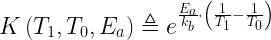
  • The interference was at 155.52 MHz – a sub-harmonic of GPON, a fiber optic transport. This relationship can be seen by noting that
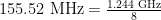
 \text{155.52 MHz} = \frac{\text{1.244 GHz}}{8}.
  • Their emergency communications were assigned to this frequency by the FCC.
  • He had not observed the interference himself, but had only heard reports of it.
  • The fire department did not have any technical knowledge of their communications system. A local consulting engineer managed the system for them.

I asked him to contact the consulting engineer and get a first-person assessment of the interference. Meanwhile, I would check with the FCC and find out what I could about their emergency communication system.

Things Begin to Clear

Once I had their radio call sign, I could use the FCC radio web site to find out information about their emergency communications system. The information would be useful in my mathematical analysis.

  • The transmitter was licensed for 100 W of effective radiated power (ERP).
  • The antenna was on a hill about one 1 km out of town (it is a small town). When I actually got on-site, I saw that the antenna could be seen from all points within the town.
  • The communication system was designed to transmit a signal that would tell scanners that it was a communication channel.

Bill had also got busy and contacted the consulting engineer in charge of their emergency communication system. Bill soon got back to me and was sounding pretty sheepish. The consulting engineer told him that the fire department had not reported ANY interference. What had been reported was that one citizen who owns a scanner was complaining that our product was causing his scanner to work differently than it had before. Prior to using our product, his scanner would scan the emergency band for fire department communications. The scanner would only stop when there was an emergency transmission. When our product had been deployed, the scanner now would constantly stop on that frequency because it would detect the low-level GPON emission from our product. Since the GPON emission from our product is no different in level from that made by a normal PC's Ethernet at \text{156.25 MHz}=\frac{\text{1.25 GHz}}{8}
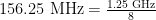
, the scanner would have trouble with or without our product being there.

The interesting thing that the consultant said was that the fire department LIKED the situation. Their communications were working fine and they consider the local citizens who monitor their communications to be a nuisance. These local folks had the nasty habit of showing up at every call the local fire department made.

While on the FCC website, I noticed that some emergency communications in my state used the same frequency as Bill's fire department. These local communities also used our product, but I had never heard any complaints from these communities. I called the folks in charge of these communications and they confirmed that they had received NO reports of interference. Now I am really confused.

What was happening here? Why was Bill's fire department having no trouble at all and the local "ambulance chasers" were unhappy? Why had no one in my state with the same situation complained at all?

A little math soon shed some light on the situation.

Analysis

Determining the Field Strength of an Isotropic Radiator

While a detailed study of the field pattern of a real antenna is complicated, we really only need an "order of magnitude" analysis to illustrate that our product could not be the source of the problem. Let's begin by deriving an expression for the field strength from an omni antenna – an omni antenna radiates equally in all directions. This will be close enough for what we are doing here. Equation 1 gives us the power radiated in all directions from an isotropic radiator.

Eq. 1 {\sigma _P} = \frac{{{P_T} \cdot {G_T}}}{{4 \cdot \pi \cdot {r^2}}}

Where

  • σP is the power per steradian (solid angle unit)
  • r is the radial distance from the antenna
  • PT is the Effective Isotropic Radiative Power (EIRP)
  • GT is the antenna gain (= 1 for an isotropic radiator)

We can use Poynting's Theorem (Equation 2) to relate the radiated power to electric field strength and magnetic intensity.

Eq. 2 {\sigma _P} = E \cdot H

Where

  • E is the electric field strength
  • H is the magnetic intensity

In Equation 3, we use the impedance of free space to relate H to E.

Eq. 3 H \doteq \frac{E}{{120 \cdot \pi }}

We can substitute Equations 2 and 3 into 1 to get Equation 4.

Eq. 4 \frac{{{P_T} \cdot {G_T}}}{{4 \cdot \pi \cdot {r^2}}} = \frac{{{E^2}}}{{120 \cdot \pi }}

We can solve Equation 4 to for E to get Equation 5, an expression for the radiated electric field strength from an omni antenna.

Eq. 5 E = \frac{{\sqrt {30 \cdot {G_T} \cdot {P_T}} }}{r}

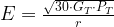
We can use Equation 5 to compare the field strength from our product to that from Bill's fire department's antenna.

Product Radiated Power Versus Fire Department Radiated Power

Field Configuation

I had been told that that problem was occuring in town. I wanted to understand how the radio signal from our product compared to that of the fire department in town. While still in the office, I used some information from Bill and Google Earth to determine that:

  • Our product was usually mounted about 30 meters from the scanner antenna
  • The fire department's antenna was about 1 km from the scanner antenna

Estimating Product Emission Level

Our product emission levels at 155.2 MHz were measured at a government-approved facility to be 30 dBµV/m at 3 meters. Since field strength varies linearly with distance from the source, the field strength from our product at 30 meters must be 1/10th the value at 3 meters or 3 dBµV/m.

Estimating Emergency Transmission Field Strengths

We can use Equation 5 to compute the field strength from the fire department's antenna. The calculation is illustrated in Equation 6.

Eq. 6 E = \frac{\sqrt{ 30 \cdot 1 \cdot 100}}{r} = \text{55,000 }\frac{\text{dB}\mu\text{V}}{m}

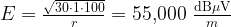
This means that the signal from the fire department is more than 17,000 times stronger than the emissions from our product. There is no way that our product is interfering with their reception. It turns out that this analysis was absolutely correct.

My Field Trip Results

When I visited Bill, things got interesting. Here is a quick summary of what I discovered on my field trip.

  • Our test gear showed that our math estimates were right on. In the town, the fire department antenna produced a monster signal compared to our product.
  • We identified emissions from our product and similar emissions from every computer, router, and switch in town. All emissions measured were within FCC limits.
  • I purchased both an analog and digital scanner so that I could see the problem myself. The analog scanner, when set at maximum sensitivity (minimum squelch), would stop scanning at 155.2 MHz when near our product. It would also stop at Ethernet emission frequencies, like 156.25 MHz, when near a PC, router, or switch. Newer digital scanners had no issue at all. Digital scanners filter out unwanted interference by identifying a special code that emergency communications systems put out. They will never lock on our product's emissions because we do not emit that special code by adjusting their squelch level up slightly.
  • It turned out that no person in Bill's community had reported any interference issues. Only one person could be found that actually had a problem and he was many kilometers outside of the city. He had an old analog receiver that was set for maximum sensitivity. This gentleman said that he needed his receiver to be at maximum sensitivity because he could just barely receive the fire department transmissions under the best of circumstances. Of course, our product had been mounted in the worst possible location with respect to interference (right next to his receiver input — 1 meter instead of 30 meters).

I now had all the information I needed to state with confidence that I had identified the root cause of the problem.

Conclusion

When I returned home I contacted my state emergency communication coordinator who informed me that my state had converted to digital emergency communications many years before. Therefore, the scanners users near my home had converted to digital scanners in the years before our products came out. There were either no more analog receivers in my area or their squelch levels had been turned up slightly to ignore the interference from any Ethernet-based product. These same squelch settings would eliminate problems with GPON emissions, too.

What happened was that Bill had one customer way out of town with an analog receiver. At his distance, the emission from our product was smaller than that of the fire department's antenna, but still large enough to be detected by his scanner (it was set at maximum gain). We informed this customer that he could try adjusting his squelch, but he refused to do that because he said increasing the squelch level would reduce his receiver's sensitivity. He felt he needed all the gain he could get to receive the fire department's signal clearly because it was weak at this distance. After reviewing his specific situation, our product had been mounted in the worst possible place relative to his antenna. We were confident that if we moved our product a few feet away from his receiver that we would eliminate the interference. Bill agreed to discuss this with the gentleman, but he was concerned that his customer may have imposed limits on where he could mount our product.

It turned out that people in town had long ago adjusted their squelch levels up to avoid interference from local computers and other Ethernet-based equipment. In fact, many of the local scanner operators had recently switched to digital scanners when their state switched to digital emergency communications. The scanner code used by the fire department was published on the web and anyone could program their digital scanner to stop only on fire department transmissions.

I told Bill that I felt that we had met our regulatory obligations and that the one person with a complaint could easily deal with the problem by moving the position of the product. Bill agreed and said that he would withdraw his complaint with the government regulator. The case was closed.

Clearly, this situation had been blown way out of proportion. Because the right people had not been put on the problem right away, actually solving the problem was taking forever and Bill had grown exasperated. In a desperate attempt to get some effective help and satisfy this one unhappy customer, Bill complained to the government. I guess his approach worked because he got me on site. As in the game "Telephone," the magnitude of the problem had grown with each retelling. By the time it got to me, it sounded like their fire department communications were totally jammed and emergency services were completely disrupted. In fact, it was an extremely minor problem with one very vocal person.

As I said in my introduction, this story illustrates my three points on dealing with field problems.

  • The first word from the field is always in error.
  • Get the right person on the problem right away or bad things are going to happen.
  • When bad things begin to happen, your ability to contain them is nil.
Posted in Electronics, Management | Tagged , , | Comments Off on The Case of the Mysterious Radio Interference

Measuring the Ring Voltage on a Telephone

Quote of the Day

Money can't buy happiness, but it can make you awfully comfortable while you're being miserable.

— Clare Boothe Luce


Introduction

Figure 1: Ringer For An Old Landline Phone.

Figure 1: Ringer For An Old Landline Phone (Source).

I received an email yesterday from a sales engineer who was having difficulty measuring the ring voltage on one of our telephone circuits. The numbers he was getting did not agree with what my engineering group had measured. The discrepancy had to do with the shape of the ring voltage waveform and what a standard voltmeter actually measures. As with many engineering problems, developing a practically useful solution depends on coming to an agreement on definitions and determining what the instruments are really measuring. This is a harder thing than one might think and this problem provides a nice illustration of basic problem solving.

Analysis

Ring Voltage Specification

The ring voltage on a telephone is specified as a Root-Mean-Square (RMS) voltage. Electrical engineers like to use RMS voltages for varying waveforms because the RMS voltage can be thought of as the equivalent DC voltage with respect to producing power in the load. Many people think of RMS voltage as a form of "average" voltage, even though it really is the average of the square of the voltage.

The Wikipedia defines the RMS voltage of a periodic signal in terms of an integral (Equation 1).

Eq. 1 {V_{RMS}} = \sqrt {\frac{1}{T}\int\limits_0^T {v{{\left( t \right)}^2}dt} }

where T is the period of the signal and v(t) is the function that describes the waveform.

Ring Voltage Waveform

Figure 2 illustrates the ring voltage waveform that the sales engineer was dealing with. Trapezoidal waveforms in telephony are common.

Figure 1: Example of a Trapezoidal Telephone Ring Voltage

Figure 2: Example of a Trapezoidal Telephone Ring Voltage

The voltage waveform actually goes both positive and negative, but the polarity does not matter when calculating power into a resistive load. We will work here with the positive side.

Computing the RMS Voltage of a Trapezoidal Waveform

Equations 2-4 illustrate how to derive and expression for the RMS voltage of a trapezoidal waveform in terms of k and T, which are defined in Figure 2. This derivation assumes that the triangular portions of the trapezoid are identical.

Eq. 2 V_{RMS}^2 = \frac{1}{T}\int\limits_0^T {v{{\left( t \right)}^2}dt} = \frac{2}{T} \cdot \int\limits_0^k {{{\left( {\frac{{A \cdot t}}{k}} \right)}^2}dt} + \frac{1}{T} \cdot \int\limits_0^{T - 2 \cdot k} {{A^2}dt}
Eq. 3 V_{RMS}^2 = 2 \cdot \frac{{{A^2} \cdot k}}{{3 \cdot T}} + \frac{{{A^2}}}{T} \cdot \left( {T - 2 \cdot k} \right) = {A^2} \cdot \left( {1 - \frac{4}{3} \cdot \frac{k}{T}} \right)
Eq. 4 {V_{RMS}} = A \cdot \sqrt {1 - \frac{4}{3} \cdot \frac{k}{T}}

Crest Factor

Just to complicate matters, the ring voltage is actually controlled by two specifications: an RMS voltage level and a Crest Factor (CF). CF is defined shown in Equation 5.

Eq. 5 CF \triangleq \frac{{\left| {\max \left( {v(t)} \right)} \right|}}{{{V_{RMS}}}}

CF is commonly used because many electronic devices are sensitive to peak-to-average ratios, which CF measures. Telephony specifications require that 1.2 ≤CF ≤ 1.6.

Correction Factor for a Peak Detecting Meter

While there are electronic voltmeters that measure true RMS voltages for any waveform, the sales engineer in this case is using an electronic voltmeter that assumes the operator is always measuring a sinusoidal signal. It measures the peak voltage of the voltage waveform and divides that value by the square root of 2, an approach which produces the correct RMS value for a sinusoidal waveform but not a trapezoid (see Equation 6).

Eq. 6 {V_{Meter}} = \frac{A}{{\sqrt 2 }}

Equations 7-8 show how to calculate a correction factor for adjusting the meters reading to give the RMS voltage for a trapezoid.

Eq. 7 {V_{RMS}} = \frac{{{V_{RMS}}}}{{\max \left( {\left| {v(t)} \right|} \right)}} \cdot \frac{{\max \left( {\left| {v(t)} \right|} \right)}}{{\sqrt 2 }}.\sqrt 2
Eq. 8 {V_{RMS}} = \frac{{{V_{Meter}}}}{{CF}} \cdot \sqrt 2

A Field Example

In this particular case, the field engineer was measuring 60 V for something that Engineering said was 65 V. We can summarize the critical variables as follows:

  • Trapezoid voltage peak voltage (A), is 86 V (set by the telephone ringer circuit design).
  • CF is 1.33 (set by Engineering in the firmware)
  • Value measured in the field, VMeter, is 60 V.

We can compute the correct RMS value by using Equation 8. This calculation is shown in Equation 9.

Eq. 9 {V_{RMS}} = \frac{{{V_{Meter}}}}{{CF}} \cdot \sqrt 2 \doteq 60{\text{ V}} \cdot \frac{{1.414}}{{1.333}} = 65{\text{ V}}

This shows that the result measured by the sales engineer and my engineering group were actually the same.

Posted in Electronics | Tagged , , | 15 Comments