Rule of 72 Redeux

I frequently have to work on “time value of money” problems. Good approximate solutions to these problems can often be obtained by using the “Rule of 72.” The Rule of 72 will tell you approximately how many interest payment intervals are required for an investment to double in value by evaluating the following formula.

N = \frac{{72}}{{r\left[ \%  \right]}}

Where N is the number of payment intervals and r is the interest rate in percentage. I just accepted this formula for years until I had a mathematician friend tell me that the Rule of 72 should really be the “Rule of 69.” He did not go into detail and I decided to think a bit more about the equation.

To determine the doubling interval of an investment, the basic equation that must be solved is the following.

{A_0} \cdot {\left( {1 + r} \right)^N} = 2 \cdot {A_0}

The exact solution is straightforward and can be derived as follows.

{A_0} \cdot {\left( {1 + r} \right)^N} = 2 \cdot {A_0}

\log \left( {{{\left( {1 + r} \right)}^N}} \right) = \log \left( 2 \right)

N \cdot \log \left( {1 + r} \right) = \log \left( 2 \right)

N = \frac{{\log \left( 2 \right)}}{{\log \left( {1 + r} \right)}} \doteq \frac{{69}}{r}

I now understand where my friend's comment came from. So I decided to graph the error in the Rule of 72 and Rule of 69 from the exact solution to see which is closer. The result surprised me.

Percentage Error Between Rule of 72 and Rule of 69 Versus Interest Rate

Percentage Error Between Rule of 72 and Rule of 69 Versus Interest Rate

Observe that the Rule of 72 has less error than the Rule of 69 for interest rates greater than 3.4%. These are common interest rates and I began to wonder if the Rule of 72 was written the way it is for a reason. Like always, I began to play with the equation. I soon saw that the Rule of 72 could be obtained by continuing the previous derivation with a slightly changed logarithm approximation.

N = \frac{{\log \left( 2 \right)}}{{\log \left( {1 + r} \right)}} \doteq \frac{{69}}{{r - \frac{{{r^2}}}{2}}} = \frac{{69}}{{r \cdot \left( {1 - \frac{r}{2}} \right)}} \doteq \frac{{69 \cdot \left( {1 + \frac{r}{2}} \right)}}{r}

We can make the error in this equation near zero for interest rates around 8% by substituting 8% in for r in numerator. The numerator function changes more slowly than the denominator function and an approximation is worthwhile there.

N \doteq \frac{{69 \cdot \left( {1 + \frac{{8\% }}{2}} \right)}}{r} = \frac{{72}}{r}

This gives us the Rule of 72 and explains why the error goes to zero for interest rates around 8%.

Posted in Financial, Management | 1 Comment

Estimating Product Cost Part 1

The Problem
I frequently am required to estimate product cost in the middle of some meeting with little or no preparation. As you gain more experience with building product, you soon are able to estimate a product's cost quickly for a production rate you are experienced with. The issue gets more complicated when you are asked to estimate product cost for production rates that you have no experience with. Unfortunately, this situation occurs far more than most engineers would care to admit. The answers are important — I have been working in start-ups where the question of product cost is critical to when you will hit profitability. You need to be able to estimate product cost at various production rates.

My Approach

I really had not thought about this question much until one day I was sitting in yet another vendor' s product cost presentation. During this seemingly endless presentation, there was a table that looked something like this.

Diplexer Cost
Component Cost Versus Volume
Annual Volume Cost
10K $100.00
20K $93.00
40K $86.49
80K $80.44
160K $74.81

This table was unusual because the price breaks occurred at points related by factors of 2. A quick check with my calculator verified that the our component costs would drop by 7% for each doubling of our annual component consumption. As I thought about it, this made sense. Doing a detailed, "bottoms-up" quote requires a lot of work. You must get quotes from all the vendors who make the parts that you must buy at the quantities that you must quote. Most of the time, customers do not end up buying at the rates they want you to estimate costs for. To make things easier, my vendors must be using a simple formula to estimatetheir product costs for the different production rates that customers were requesting. As it was for me, it is hard for them to constantly ask their vendors to quote on quantities that will never be ordered.

This prompted me to try the following cost model for all my components.

{C_N} = {C_R} \cdot {(1 - r)^{lo{g_2}\left( {\frac{N}{R}} \right)}}

Where CN is the component cost at a production rate of N, CR is the reference production rate R (say 10K per year), and r is the discount rate per doubling. In real life, price breaks occur at discrete points. However, a continuous model is useful for cost estimation purposes.

This model almost always worked for component consumption rates less 100K units per year. I found that the discounting rates varied from 5% to 10% per doubling of annual component consumption. I also applied the model to the overall product cost and found that my total unit product cost reduced in cost by an average of 7% for each doubling of annual production rates. I have used this model for the last 10 years with good agreement with reality.

This has proven to be a useful way to estimate how product cost varies with annual production rates. To illustrate how to apply this approach, let's work through an example.

Example

I often tell people that when it comes to manufacturing cost, the manufacturer with the highest production rates wins the game ("he with the most volume wins"). In a recent meeting, I was told that a competitor is reporting similar margins to ours, but his average selling price is 21 % lower than ours. His annual volume is 8x our annual volume (2^3 or 3 doublings). I responded that based on volume alone, our competitor has a 21% cost advantage over us. After discussing the situation for a while, everyone in the room agreed that a product cost advantage of ~20% would explain what we were seeing.

A Competing Model
Armed with my observation, I figured someone else has seen this relationship. I found only one article on the Internet that mentioned that PC costs were seen to drop by 10% for every doubling of volume. So this characteristic has been observed in other markets.

Further research showed me that there was another relationship that was also common. It used the following model.

{C_N} = {C_R}\cdot{\left( {\frac{N}{{{N_R}}}} \right)^q}

Where q is a parameter that varies for each product. This model matches mine in performance exactly. It turns out that we can show that both models are equivalent. I prefer my approach because I can estimate the discount rate by simply estimating the number of doubling over the reference rate and multiplying by 7%.

Equivalence Demonstration

I will begin with the form of the equation that I use and step-by-step get to the alternate form.

{C_N} = {C_1}\cdot{\left( {1 - r} \right)^{lo{g_2}\left( {\frac{N}{R}} \right)}}

{log_2}\left( {{C_N}} \right) = {log_2}\left( {{C_1}} \right) + {log_2}\left( {\frac{N}{R}} \right) \cdot {log_2}\left( {1 - r} \right)

{log_2}\left( {{C_N}} \right) = {log_2}\left( {{C_1}} \right) + \left( {{log_2}\left( N \right) - {log_2}\left( R \right)} \right)\cdot{log_2}\left( {1 - r} \right)

{log_2}\left( {{C_N}} \right) = {log_2}\left( {{C_1}} \right) - {log_2}\left( R \right) \cdot {log_2}\left( {1 - r} \right) + {log_2}\left( N \right)\cdot{log_2}\left( {1 - r} \right)

{C_N} = {\text{ }}\frac{{{C_R}}}{{{R^{{{\log }_2}\left( {1 - r} \right)}}}}\cdot{N^{lo{g_2}\left( {1 - r} \right)}} = {C_1}\cdot{N^q}

The derivation can be reversed to convert the alternate form to my form. Thus, the forms are equivalent.

Extending the Model

I mentioned that this model works for production volumes less than 100K. For higher annual production volumes, the rate of cost reduction reduces. For my products, I have seen the discount rate decrease from the 7% to 2% per doubling on production rates higher than 100K per year. The exact annual production rate and discount rate breakpoints vary by vendor.

Real Component Pricing Example
There is often some strategy used in the pricing of components. Here is a table product pricing table from a vendor that shows a bit of strategy being used. The vendor figured out that my total annual usage of this part was about 100K. He wanted all of our business, so he gave us a quote that was high for annual rates less than 100K but low for rates greater than 100K. Basically, he wanted to ensure that we would be tempted to make him the sole source on this part. Because of this strategy, my pricing function does not apply as well to this situation.

Optical Component Cost
Component Cost Versus Volume
Annual Volume Cost
1K $14.40
10K $13.34
50K $12.56
100K $11.38
250K $11.08
500K $10.68
1000K $10.29

You can see the discontinuity in the cost function on the following chart.
Plot of table data

Posted in Management | Comments Off on Estimating Product Cost Part 1

The Capacitor Puzzle That Got Me My First Job

In the spring of 1979, I was a soon-to-be-graduated electrical engineer that needed a job. As with other young engineers, I started to look for work during my last semester of school and I got a few nibbles. The most intriguing of the nibbles was from Hewlett-Packard, known by all engineers as "HP." At that time, HP was considered a class engineering act and getting a job there would be perfect for someone with plenty of energy but little experience.

The first interview was on campus and was pretty interesting. HP was known for having a tough on-campus interview. They asked tough questions. The questions weren't necessarily technical – most were puzzles. Fortunately, I like puzzles!

The interview went well and they sent me a plane ticket to Ft. Collins, Colorado for an interview. Soon I was out in Colorado. It was the first time I had flown (excluding one quick flight on a Piper Cub when I was 7). It was also the first time I had stayed at a motel without my parents. It was a trip filled with firsts for the kid from small-town USA!

The interview ended up being a grueling six-hour puzzle-solving session. Once I got over my initial jitters, I relaxed and actually enjoyed the experience. It must have gone well because I received a job offer before I left the building.

During my interview, there was one problem that kept coming up. It turned out the problem had been the subject of much discussion within HP. The Fort Collins facility was filled with engineers who loved math puzzles, which made sense when you think about their interview process. If you hire based on the ability of people to work puzzles, you probably end up hiring people who are good at them.

The problem begins with a young engineer being handed a 1 F (Farad) capacitor that is charged to 10 V.

You are handed a 1 F capacitor charged to 10 V and two boxes containing uncharged capacitors: one box contains an uncharged 1 F capacitor and the other contains 1 million 1 µF capacitors. You can connect the capacitors from one box, one at a time, across the charged capacitor. Your job is to determine which box will allow you to discharge the voltage on the charged capacitor the most?

Consider the first box. You can think of a 1 F capacitor as one million 1 µF capacitors in parallel. When this capacitor is connected across the charged capacitor, the final voltage will be 5 V and every capacitor will have the same voltage. The following figure illustrates the situation.

Now consider the box of one million capacitors. The first small capacitor you apply will be charged to nearly 10 V because the capacitor being connected is so small compared to 1 F.
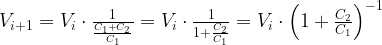
We can compute the voltage on the 1 F capacitor using the definition of capacitance. Let {C_1} = 1\;{\text{F}}. We can write the following equations.

{V_i} \cdot {C_1} = {V_{i + 1}} \cdot \left( {{C_1} + {C_2}} \right)

{V_{i + 1}} = {V_i} \cdot \frac{1}{{\frac{{{C_1} + {C_2}}}{{{C_1}}}}} = {V_i} \cdot \frac{1}{{1 + \frac{{{C_2}}}{{{C_1}}}}} = {V_i} \cdot {\left( {1 + \frac{{{C_2}}}{{{C_1}}}} \right)^{ - 1}}

This equation can now be applied one million times to determine the final voltage. Of course, applying this equation one million times means that we will be close to the limit of the following equation. So let's go find the limit.

{V_\infty } = \mathop {\lim }\limits_{\frac{{{C_2}}}{{{C_1}}} \to 0} \quad 10\;{\text{V}} \cdot {\left( {1 + \frac{{{C_2}}}{{{C_1}}}} \right)^{ - \frac{{{C_1}}}{{{C_2}}}}}

To simplify my notation, let n \triangleq \frac{{{C_2}}}{{{C_1}}}. We can then write

{V_\infty } = \mathop {\lim }\limits_{n \to 0} \quad 10\;{\text{V}} \cdot {\left( {1 + \frac{{{C_2}}}{{{C_1}}}} \right)^{ - \frac{1}{n}}}

When I looked at this equation, I realized that this was the equation for continuous compound interest. While in school, I had seen this limit and I was able to write down the answer directly.

{V_\infty } = 10 \cdot {e^{ - 1}} = {\text{3}}{\text{.678796}}

So the answer to the question of whether to choose box one or two was clear ─ choose box 2 with one million 1 µF capacitors. The capacitors will end up charged as shown below.

My interviewer looked stunned. He asked how I knew this and I told him that I had seen the limit before. He looked dismayed and said that he would prefer to see a method that did not require a "miracle" of observation. Our interview time was then over and I had another interviewer to face. Later that day I would receive a job offer and would return to live in Ft. Collins a few months later.

When I arrived in Ft. Collins to start my job, one of my interviewers came up to me and asked if I could come up with a more satisfying solution (i.e. one that did not require identifying the series by inspection).

As I looked at the equation, I told my interviewer that l'Hôpital's rule could probably be applied. My interviewer said that l'Hôpital's rule did not apply to equations of this form. Fortunately, I had recently seen a professor solve a similar problem by applying l'Hôpital's rule's to the logarithm of this equation. It turned out that l'Hôpital's rule could be applied to the logarithm of this equation.

\ln ({V_\infty }) = \ln (10) + \mathop {\lim }\limits_{n \to 0} \left( { - \frac{{\frac{d}{{dn}}\left( {\ln \left( {1 + n} \right)} \right)}}{{\frac{d}{{dn}}\left( n \right)}}} \right)

\ln ({V_\infty }) = \ln (10) + \mathop {\lim }\limits_{n \to 0} \left( { - \frac{{\frac{1}{{1 + n}}}}{1}} \right)= \ln (10)-1

{V_\infty } = 10 \cdot {e^{ - 1}} = {\text{3}}{\text{.678796}}

The interviewer looked at me with both happiness and dismay. He said that he had been working for months off and on trying to analytically come up with the limit. He also mentioned that my puzzle-solving ability was what motivated them to hire me.

Ever since then, I have fondly thought of this math puzzle. It is hard to believe that it got me my first real job!

Posted in Interviewing, Problems | Tagged , , , | 20 Comments