
Quote of the Day
Everything comes to he who hustles while he waits.
— Thomas Edison
Introduction

Figure 1: Image of CVSO30c From The
Very Large Telescope in Chile (Source).
I saw an article in the popular science press about a real rarity – an exoplanet that can be seen (Figure 1). I dug around the web and found the journal article on which most of the press articles were based. Given their measurement data, I wanted to see if I could duplicate some of their computed exoplanet characteristics. In this post, I will be using some of the techniques learned about while listening to The Search for Exoplanets: What Astronomers Know.
Much of the data that astronomers are gathering is obtained using the transit method of exoplanet detection. While this is a powerful technique, it can only be applied to about 0.5% of the star systems we can view – systems that are edge-on to our field of view and where eclipses can occur. While not a general method, the transit method has been used by the Kepler spacecraft to find over 1000 confirmed exoplanets, which is impressive considering that considering that Kepler stares at a fixed set of ~145K stars (i.e. a tiny portion of the sky).
I include a copy of my Mathcad source here.
Background
Reference Material
I have covered exoplanet detection and analysis methods in other posts. Here is a list of my previous posts:
- Discussion of the Kepler satellite, which has demonstrated the power of the transit method of exoplanet detection.
- Discussion of how the transit method can be used to determine some important exoplanet characteristics.
In this post, I will show how the effective temperature of the exoplanet can be used to estimate its radius. One interesting development is that the basic transit method is now being extended to provide some atmospheric measurements. These measurements can be used to estimate the surface gravity of the exoplanet, which in turn can be used to estimate the mass.
For planetary systems that are close to ours, astronomers can use transit and radial velocity methods to cross-check their estimates. This also helps to reduce the effects of systematic errors.
Star/Planet Information Information
The journal article mentioned above provided the following measurements of CVSO30 and CVSO30c.

Figure 2: Key Measurements from Transit Observations.
I should point out that some of these measurements are based on spectra (e.g. surface gravity), which requires quite a bit of light to generate. As I mentioned in this post, the amount of light available from even nearby stars dribbles in at a handful of photons per second. This makes these measurements very time consuming.
Analysis
Utility Functions
Figure 3 shows the basic astronomical formulae needed to compute some exoplanet characteristics. Note that I did not include the formula for estimating the distance between the exoplanet and star, 
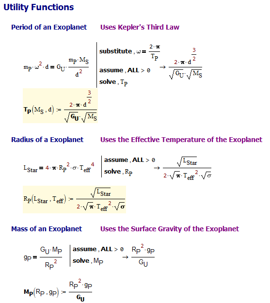
Figure 3: Utility Functions.
Analysis Setup
Figure 4 shows all the units and constants I used for this analysis. The values all came from the Wikipedia.

Figure 4: Units and Constants.
Solution
At this point, all I need to do is substitute the measurements into the utility functions. Figure 5 shows the results of these calculations. My results are very close to the values in the referenced journal article.
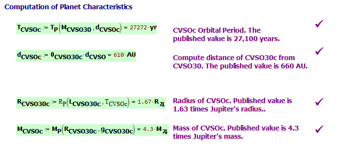
Figure 5: My Results Using the Observational Data.
Conclusion
This was the first time I had seen that astronomers could measure the surface gravity of an exoplanet and use that value to estimate the exoplanet's mass. The use of the exoplanet's effective temperature is also interesting because it can be used to determine the radius of the exoplanet.