Quote of the Day
We live in a world where not everyone has the urge to help others… It is OK to encourage others to pull themselves up by the bootstraps, but if you do, just remember that some people have no boots.
— Neil deGrasse Tyson. My father used to make a similar statement. He always wanted to help others.
Introduction

Figure 1: Typical News Report of Venus-Like Exoplanet (Source).
I have been reading a number of articles that are reporting on a Venus-like planet (GJ 1132b) recently discovered in a nearby red dwarf star system (Gliese 1132, 12.0 parsecs away). I like to work a bit with the numbers reported in these articles to determine if I actually understand what is being reported. I have to admit that I also like to imagine the day when astronomers are studying Earth-like planets around other stars. I definitely see that day coming. Discoveries like GJ 1132b are particularly interesting because astronomers for a long time did not think red dwarf stars were promising for Earth-like planets.
All the data being reported in the new reports appears to come from a single journal article. The articles have all made statements similar to those in this list:
- The planet has an average surface temperature of 450 °F.
- The planet has a diameter of 16% larger than the Earth (9200 miles)
- The planet has a density of 6 grams/cm3.
- The planet was detected using the transit photometry, which detected a 0.26% drop in the light output of the star when the planet passed in front of the star.
My goal here is to understand how these estimates were based on the observations the astronomers actually made.
Background
The star, Gliese 1132, is a red dwarf star that I will assume to have the following characteristics:
- 20% of our Sun's luminosity
- 20.7% of our Sun's diameter
- 18.1% of our Sun's mass
Astronomers have well-established methods for determining these parameters, which I will not cover in this post – they will be fodder for a future post.
There really are only two measurements associated with the planet itself.
- The star had a radial velocity of 2.7 m/s
The radial velocity is the speed that object moves away from or approaches the Earth. We can measure this speed very accurately using the Doppler shift. This radial velocity is related to the momentum of planet that is orbiting the star, which you can see in Figure 2.

Figure 2: Illustration of Star's Radial Velocity. The star is the large body in the center (source).
- There was dip of 0.26% in the star's light level that occurred with a 1.63 day period.
We can illustrate the dip in light level as shown in Figure 3.

Figure 3: Illustration of Light Level Dip Due to Planet Transit.
The original paper included error ranges about each measurement, which I will ignore for my rough work here. As I show below, these measurements can be used to learn much about the planet that circles this star.
Analysis
Planet Orbital Radius and Mass
Figure 4 shows my calculations for the planet's orbital radius and mass. The approach I used is described in the Wikipedia and this document, so I will not go through the formulas further. I will say that if you look carefully, you will see Kepler's 3rd Law, i.e.  . As I show in Figure 2, my calculations are almost identical with those reported in the original paper.

Figure 4: Planet Orbital Radius and Mass.
In Figure 4, I determine the planet's mass using the fact that the star's momentum and the planet's momentum must be equal. Figure 5 illustrates this fact.

Figure 5: Illustration of Star and Planet Momentum, Which are Equal.
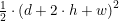
Planet Diameter
Figure 6 shows how you can compute the diameter of the planet using the measured dip in the Gliese 1132's light output as the planet passes between Earth and Gliese 1132, an approach that is known as the Transit Method. The diameter estimate assumes the light occulation is proportional to the circular area ratio of the planet to the star Gliese 1132.

Figure 6: Computing the Diameter of the Planet.
Planet Density
Since we have the planet's mass and diameter, we can compute the density of the planet as shown in Figure 7.

Figure 7: Calculation of the Planet's Density.
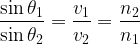
Planet Temperature
Figure 8 shows how we can compute the temperature of the planet, assuming no greenhouse effect. The technique is described well in the Wikipedia and I will not say more here.
You can see that the temperature estimate is strongly affected by the assumptions made about the planet's bond albedo – the fraction of power in the total electromagnetic radiation incident on an astronomical body that is scattered back out into space. My results are virtually identical to those reported in the original paper, which assumes a range of bond albedo's from 0 to 0.75. The news articles all chose different temperature values within the range reported by the original paper.

Figure 8: Estimate of the Planet's Temperature.
I should mention that the same calculation performed on the Earth would show that our average temperature should be around -17 °C (see Appendix A). However, the actual mean temperature of the Earth is ~16 °C (source). The difference is because of the greenhouse effect.
Conclusion
With a bit of basic physics, I was able to reconstruct the derived exoplanet characteristics presented in the original paper. I always find it amazing how much information we can derive about a planet with just a few numbers and no direct visual observations.
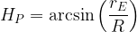
Appendix A: Calculation of Earth's Temperature Assuming No Greenhouse Effect.
You can find the Earth's albedo value here. Figure 9 shows the calculation.

Figure 9: Earth's Mean Temperature Assuming No Greenhouse Effect.
The actual mean temperature of the Earth is ~16 °C. The difference of 33 °C is because of the greenhouse effect.