People of mediocre ability sometimes achieve outstanding success because they don't know when to quit. Most men succeed because they are determined to.
— George Allen
Introduction

Figure 1: Bicycle as Projectile (Braden Hanna).
In our previous post, we developed an expression for y' (=dy/dx, Newton's notation) expressed as differential equation in terms of x. We will now solve this equation through the use of an integrating factor. Having solved for y' in terms of x, we can integrate that expression to obtain y(x).
The exact expression for y(x) is a bit complex and Pejsa spent a quite a bit of book space developing a good approximation for y(x) that is both accurate and simple. In this post, we will derive both the exact and approximate solutions.
Background
Pejsa's Approximate Solution
Our goal in this post is to derive Equation 1, which is Pejsa's approximate solution to his projectile drop equation that we developed in Part 1.
| Eq. 1 | 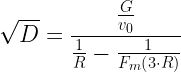 |
where
- D is the projectile drop [inches]
- v0 is the initial projectile velocity [ft/sec]
- R is the projectile horizontal travel distance [yards]
- G is a constant with value 41.697 [ft[sup]0.5[/sup]/sec]
- Fm (R)= F0-3·n·R/4 (I call this the "standard form")
Pejsa uses the subscript "m" to stand for "mean". I should mention that while Pejsa's derivation uses this formula, his actual software uses the following modified form
(I call this the modified form). He has a worked example on page 94 that also uses the results from the modified Fm , with no prior warning of a change. I spent many hours trying to find the discrepancy. I assume that he made this change to improve his approximation a bit, which I demonstrate in Appendix A.
Analysis
Solving For y'(x)
Figure 2 shows how we can use an integrating factor to solve the differential equation for y' as a function of x.

Figure 2: Solving The Differential Equation for y'.
Solving For y(x)
Figure 3 show how we can integrate y'(x) to obtain an exact solution for y(x).

Figure 2: Integrating y' to Obtain y.
From my standpoint, the exact solution is reasonable for implementation using either software and spreadsheets. I agree that it would be painful if all you had was a 1970s–era calculator.
Approximation
Figures 4 and 5 show how Pejsa used a Taylor series approximation of the exact solution to obtain a computationally-easier result that provides good agreement for typical projectiles (i.e. ballistic coefficients from 0.3 to 0.5 [Pejsa, page 143]).

Figure 4: Developing a Taylor Series Approximation.

Figure 5: Approximate Solution With No Unit Assumptions.
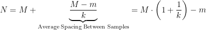
Standard Form of Pejsa Approximate Solution Assuming US Units
Figure 6 derives the most commonly seen form of Pejsa's approximate solution using US customary units.

Figure 6: Approximate Solution Using US Customary Units.
Conclusion
Now that we have developed both the exact and approximate solutions, I will work an example in part 3. An example is definitely needed.
Appendix A: Error Between Exact and Approximate Solutions
Figure 7 shows a plot of the percentage error between the exact solution and the approximate solutions (standard and modified Fm) for a projectile with a ballistic coefficient of the 1 (I will discuss ballistic coefficients in part 3). Observe that the errors are small for both forms of Fm, but the modified Fm is distinctly better.

Figure 7: Plot of Errors Between Exact and Approximate Solutions.

 . It will be used in deriving the projectile drop differential equation, but will not play a significant role in its solution.In his book, Pejsa sometimes uses A to represent acceleration. This created some confusion for me as I read the book. In these posts, I will make sure that A is only used to represent the proportionality constant.
 , which I will use in the mathematical development to follow.
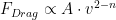 .
.