This Idea Solves a Life-Long Problem

Quote of the Day

Beware the fury of the patient man.
— John Dryden


I cannot tell you how often in 35 years of marriage I have come home to the open-ended question from my wife "Do you like it?", without "it" being defined. I then spend the next 10 uncomfortable minutes trying to figure out what aspect of my wife's appearance has changed. I admit that I simply do not notice things like haircuts, changes in hair color, new clothes, etc. I am so bad that I have even failed to notice a complete change of hair color (blonde to brunette).

I saw the following absolutely brilliant post on Reddit this morning.

I know a guy who has a standing $10 tip with his wife's hair dresser. He gets a call each time his wife gets her hair cut with a brief description of what was done. Wife walks in the door, he says "Honey, did you get your hair done? It's a bit shorter and looks great!" Winners all around.

I know my wife's hairdresser (good friend of both of us) and I think I can make this work. It may not solve all my issues with noticing things, but it will solve the hair part.

Posted in Personal | Comments Off on This Idea Solves a Life-Long Problem

Calibrating My Chop Saw to Make a Perpendicular Cut Using a Bit of Geometry

Quote of the Day

All heiresses are beautiful.

- John Dryden


My co-workers and I are pretty serious DIYers so we always talk about new projects and tools we're getting into. In fact, the last few weeks has consisted of us trying to find the best 90 degree drill because one of them is about to start a project that's in a lot of tight spaces. But, no matter how much we talk about them, we don't know if we're going to like the power tools when we try them out and one of my co-workers was very disappointed with his purchase of a DeWalt DW717 miter saw because it does not make a perpendicular cut. Figure 1 shows a picture of his saw.

Figure 1: DeWalet DW717 10-inch Miter Saw.

Figure 1: DeWalt DW717 10-inch Miter Saw.

A little while ago I needed to get a miter saw for a project I was doing. I did my research and decided to choose a cordless miter saw over a corded one because then I wouldn't be restricted. This means that I have a similar saw (12-inch version) and I am very happy with mine. I thought for a moment and asked my co-worker "Have you calibrated your saw?" He told me, no and he did not know it could be calibrated. Time for a little geometry -- construction always presents me with the best classical geometry exercises.

Very few tools come from the factory accurately setup -- at least to the accuracy I expect. I regularly calibrate both the 90° and 45° settings on my miter saw. In today's post, I thought I would show how I calibrate my saw for perpendicularity (i.e. 90° cut). I will discuss how to calibrate for a 45° cut in a later post. Figure 2 illustrates my approach. I was taught this in my youth and I do not remember by whom -- my dad spent all day at a saw cutting wood with a DeWalt saw and I think he might have taught me. He loved DeWalt and I think of him every time I use a DeWalt product.

Figure 2: My 90° Calibration Process.

Figure 2: My 90° Calibration Process.

My co-worker went home and proceeded to tune up his saw nicely. He is now a happy woodworker.

Posted in Construction, Geometry | Comments Off on Calibrating My Chop Saw to Make a Perpendicular Cut Using a Bit of Geometry

My ANOVA and Gage R&R Self-Education

Quote of the Day

Who are a little wise the best fools be.

— John Donne


Introduction

Figure 1: Calipers, A Form of Gage.

Figure 1: Calipers, A Form of Gage.

I recently took an excellent class at Statistics.com called "Prediction & Tolerance Intervals, Measurement and Reliability" taught by Dr. Tom Ryan, a former NIST researcher. I took the class because I have been concerned that some of the statistical methods I am currently using for calibrating optics are not as good as they could be. As part of the class, we were required to perform some practice Gage Repeatability and Reproducibility (aka gage R&R) studies, which required me to use ANOVA. The class gave me many ideas for improving my experiment design and I highly recommend it to those who do a lot of experiments.

Figure 1 shows a caliper, which is a common form of gage (sometimes spelled gauge). A gage is any device that is used to perform a measurement. In my case, I will be performing gage R&R on some optical power measurements.

In this post, I am focusing on my self-education on ANOVA and its application to gage R&R. While I have used ANOVA for years for evaluating the significance of test data, but I have never looked at how it works until very recently. The opportunity to study ANOVA in detail came because of some work I needed to do in Taiwan (a place that I enjoy very much). On the flights from Minneapolis to San Francisco to Taiwan, I had 17 hours of flight and a 5 hour of layover to think about how ANOVA works. I put this time to some good use.

Background

Source Material

My approach here will slavishly follow that of M.J. Moroney in his excellent book "Facts From Figures". First published in 1951, you can find this book in used bookstores for about $1 or you can download it in PDF form from the web. I discovered this little gem years ago and I turn to it when I need a short refresher on basic statistics.

Why Gage R&R?

When I started my career at HP back in 1979, my mentor there told me that "Manufacturing is in a constant battle against variation -- ideally, we make the millionth unit the same as the first." To battle variation, we must first be able to identify and measure it. The focus of gage R&R is on understanding and measuring the sources of variation in a measurement. Because good product design practice requires that you design for the worst-case parameter variation, excessive variation in measurement forces you to design your product to be tolerant of this variation and that increases cost.

The folks in our Quality team break down variation as shown in Figure 2 (Source).

Figure 2: Components of Variation.

Figure 2: Components of Variation.

When we talk about measurement variation, we are talking about precision. The Wikipedia describes precision as follows

The precision of a measurement system, related to reproducibility and repeatability, is the degree to which repeated measurements under unchanged conditions show the same results.

Gage R&R explicitly measures reproducibility and repeatability relative to the level of part variation.

Approach

Most technical discussions of ANOVA dive into equations with multiple levels of summation symbols. Moroney begins his example by taking a simple experiment and showing how you can can break the variance of the result into components with no use of summations. I like this approach as a gentle start.

Since I am focused on gage R&R here, my plan is produce a several related worksheet items all contained in a single Excel workbook (available here) that does not use any Visual Basic. :

  • An Excel worksheet that works through one of the ANOVA examples from "Facts From Figures". While not a gage R&R example, I will use this example as the basis of my gage R&R work. Here is the book excerpt that I am using as my gage R&R reference.

    The examples in this book are simple because they are from a time when calculations were done by hand. This is not a bad thing for today because it means you can easily duplicate them using a tool like Excel or Mathcad. While I prefer to use Mathcad for nearly everything, Excel is probably a better vehicle for my study work here.

  • A set of Excel worksheets that contain gage R&R example using a template I have created whose results agree with the same data processed by Minitab, which is the tool Dr. Ryan recommended (he was one of its creators).

    Yes, Dr. Ryan strongly discouraged me from using Excel for ANYTHING, but I do believe it can play a role in routine statistical calculations and I will ignore his advice here. As you can see, I often do not follow directions. Sister Mary Agnes from the Osseo Catholic School is probably looking down upon me from heaven with a frown on her face.

This worksheet is intended to illustrate the concepts behind ANOVA and gage R&R -- it is not computationally efficient. However from a conceptual standpoint, I like Moroney's approach of eliminating row and column variation in separate operations to determine the desired variance components.

Analysis

Role of ANOVA in Gage R&R

ANOVA is one of the accepted methods for determining the variance components in a experiments (cf. AIAG approach). With respect to this post, there are three sources of variation: the part itself, the operator, and random error. Gage R&R studies often include modeling the interaction between part and operator, but to keep things simple I will ignore this sort of variation for this post. The methods shown here can be extended to include interaction, but I want to keep this post simple.

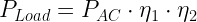
Equation 1 shows the gage R&R variance model that I will be using.

Eq. 1 \displaystyle \sigma _{T}^{2}=\sigma _{Reproducibility}^{2}+\sigma _{Parts}^{2}+\sigma _{Repeatability}^{2}

where

  • σT2 is the total variance of data.
  • σParts2 is the component of variance due only to the parts.
  • σReproducibility2 is the component of variance due only to the operators.
  • σRepeatability2 is the component of variance due only the measurement tools.

We will use ANOVA to determine the variance components. Once we have the components, we can determine the relative effects on our measurement of the different components. Customarily, we want to see the repeatability and reproducibility components to be less than 10% of the total variance (example of the 10% standard).

My ANOVA Reference Model

Figure 3 shows my rework of Maroney's Latin Square excerpt, which is focused on "treatments" applied to some crop. This is the example I used as my model for writing a simple gage R&R worksheet. The process for generating Figure 2 can be broken down as follows:

  • Average the effect of each set of treatment levels, then determine the Mean Square error (MS) of the treatment.

    We will use this term to estimate the variance contribution of the treatment.

  • Remove the effect of row variation by replacing each row element with the average element value for that row.

    By eliminating the row variation, we can compute the MS of the column variation.

  • Remove the effect of column variation by replacing each column element with the average element value for that column.

    By eliminating the column variation, we can compute the MS of the row variation.

Figure 3: Maroney Example of Blocked ANOVA.

Figure 3: Maroney's Example of Blocked ANOVA.

My Gage R&R Worksheet

I have put a number of tabs in this Excel worksheet that duplicate the results obtained from Minitab and other tools. We can make a direct analogy between my gage R&R and Figure 3 as follows.

  • treatments in Figure 3 are comparable to parts in gage R&R. Our analysis will provide us with the part-to-part variation.
  • column variation is Figure 3 is comparable to repeatability variation in gage R&R (statistics folks will often call this term the residual error)
  • row variation in Figure 3 is comparable to reproducibility or operator variation in gage R&R.

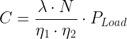
The worksheet uses array formulas to compute the gage R&R of data placed into the data area at the bottom of the worksheet. The variances are computed by substituting the MS values into the equations shown in Figure 4.

Figure 4: Equations Used For Computing Variance Components.

Figure 4: Equations Used For Computing Variance Components.

I will not be deriving the formulas of Figure 3 in this post. You can find them in various places on the web. Here is a link to one Powerpoint presentation that gives these formulas, but with different variable names. I intend to derive them in a later blog post.

Conclusion

I finally feel like I have an intuitive model of what is going on when I perform an ANOVA analysis. While you do not need to know the details of how the computation is performed, it does help you get some insight into the ANOVA process. This reminds me a bit of Fourier analysis. You do not necessarily need to know the details of a Fast Fourier Transform (FFT), but knowing the details does give you some insight into what is going on.

Posted in Statistics | 2 Comments

Repairing My Electric Dryer and a Little Math

Quote of the Day

Intentionally adding value to others today will bring you fulfillment every day.

- John C. Maxwell


I came home the other night and my wife reported that our clothes dryer was not generating any heat for drying clothes. I had heard a few people having the same issue of the dryer not heating so I did some research for myself. She called a repairman and he could not repair our dryer for a long time and was going to charge a lot of money (e.g. $90 for a heater coil that was $30 from Amazon). There was no way we could have waited, so I decided to create the beste wasdroger for her with my handyman skills.

While I know NOTHING about clothes dryers, I decided to try to fix it myself. I'll give you folks a statutory warning! If you don't have any prior experience, you could seek professional help like https://barnettelectrical.com/oklahoma-city-ac-repair/, which specializes in providing electrical services and repairs. Now coming back to my story, as with most of my repair adventures, I started with Youtube. After a couple of minutes, I found the following video where a repairman gave a great demonstration on how to change the heater coil (Whirlpool part number 3387747) in my clothes dryer.


Unfortunately, this video did not tell me how to test the dryer's heater coil -- from the schematic, it seems like a failed thermostat or thermal cutoff would also result in no heat. I decided to measure the resistance of the coil in my dryer and I discovered that the coil was open -- my heater coil had failed.

While the coil was open and clearly failed, I became curious as to what value the coil resistance needed to be. The manual for my dryer does not give me the required coil resistance, but I was able to estimate what the coil resistance should be using Equation 1 -- the formula for the power dissipated in a resistor. The only information I needed were the wattage and voltage ratings of the coil, which were stamped on its side.

Eq. 1 \displaystyle {{P}_{Coil}}=\frac{V_{AC}^{2}}{{{R}_{Coil}}}\Rightarrow {{R}_{Coil}}=\frac{V_{AC}^{2}}{{{P}_{Coil}}}=\frac{{{\left( 240\text{ V} \right)}^{2}}}{5400\text{ W}}=10.7\Omega

Figure 1 shows my failed heater coil. I found the break in the coil right away (marked in red and pulled up).

Figure 1: My Broken Heater Element. I have bent the break to make it more obvious.

Figure 1: My Broken Heater Element. I have bent the break to make it more obvious.

I ordered a new coil from Amazon and it had a resistance of 9.9 ?. My rough analysis in Equation 1 was pretty close. I also measured the resistance of my old coil (after connecting the broken pieces back together) and got 11.5 ?.

I later found another heater coil repair video that discussed how to test the heater coil. I have included this video below. This was a lifesaver! And I have since thought about getting added protection for my clothes dryer and all of my other appliances in the form of a home warranty plan (check it out here) so I don't have to worry about doing any repairs again in the future. Whilst I managed to do it successfully this time (I think), I'm not sure if I will have the same luck in the future, so it's better to have a back-up option in case anything were to go wrong.

Posted in General Mathematics | Comments Off on Repairing My Electric Dryer and a Little Math

Coaxial Cable Basics

Quote of the Day

Good intentions will never take you anywhere you want to go. Only intentional living will get you the things you want in life.

- John C. Maxwell


Introduction

Figure 1: Different Types of Coaxial Cable.

Figure 1: Different Types of Coaxial Cable.

A big part of my job revolves around cables so it's fair to say that I have a lot of knowledge about them. Whether it's using wrap around cable labels to make maintenance easier or replacing broken cables or informing customers about basic cable management. Why am I telling you this? Because I am preparing some customer education material on coaxial cables for customers (Figure 1 shows some coaxial cable examples) and I thought this information was worth documenting here. Our fiber optic products interface to coaxial cables so that service providers can use existing in-home wiring. If you are looking for a cable supplier, you can check out Sava who has a wide range of various cable types, that can be used for differing electrical needs.

Coaxial cable is much more commonly used in the United States for residential interconnect than in the rest of the world -- about 90% of US homes have coaxial cable already wired within them. In my opinion, it is also the most misunderstood of the broadband interconnection products. However, not all homeowners are aware of all of their options when it comes to cable. In fact, many end up saying things like 'I only thought there were a few cable providers in my area' when there is actually a lot more than you'd think. That is why it is always wise to shop around before committing to one particular provider.

My intent here is to cover some of the basic math associated with two important coaxial cable parameters. In later posts, I will discuss how the temperature affects coaxial cable losses and length, which are the specific topics that I am addressing with customers this week.

Background

Construction of Coaxial Cable

Figure 2 shows a section drawing of coaxial cable.

Figure X: Coaxial Cable Cutaway Drawing.

Figure 2: Coaxial Cable Cutaway Drawing.

Figure 3 nicely shows how a typical coaxial cable is constructed (RG-59 in this case). RG-59 and RG-6 cables are very similar. RG-59 is cheaper and media equipment manufacturer's (e.g. like for TV and DVD players) often include it with their gear for use with short interconnections because it is cheaper than RG-6. RG-6 has a heavier core conductor and better shielding, so it works better for longer runs.

Figure X: Appearance of a Typical Coaxial Cable.

Figure 3: RG-59 Coaxial Cable Components: (A) Outer plastic sheath, (B) Copper braid shield, (C) Inner dielectric insulator, and (D) Copper or copper-plated core (Source: Wikipedia).

Types of Coaxial Cable

Here is a good article on some common types of coaxial cable. However, this post will focus on RG-6, which is commonly used in residential analog video deployments (e.g. NTSC). My questions from the field are nearly always about RG-6 cable. As analog video vanishes, the in-place coaxial cable is being re-purposed to carrying digital video using MoCA and HPNA. So we are going to see the residential use of coaxial cable for a long time.

History of Coaxial Cable Impedance Values

I found some interesting articles that discussed the history of 50 ? and 75 ? characteristic impedance values for coaxial cables:

Analysis

From my standpoint, the two most important electrical characteristics of coaxial cable are:

  • Characteristic Impedance
  • Attenuation

I will use a couple of common formulas for estimating these values using two different types of RG-6 cables. I will not attempt a derivation because the good folks at Microwaves101 have done a great job documenting the formulas for both characteristic impedance and attenuation.

Characteristic Impedance

Figure 4 shows how the mechanical construction of an RG-6 cable determines its characteristic impedance. For my example cable, I used the Belden 1694A. Figure 4 assumes that µR = 1, which is true for most non-ferrous materials (link).

Figure 4: General Formula for the Characteristic Impedance of a Coaxial Cable.

Figure 4: General Formula for the Characteristic Impedance of a Coaxial Cable.

My calculations show a 74 ? characteristic impedance for this cable, which is very close to the manufacturer's stated 75 ?.

Attenuation

Figure 5 shows how the mechanical construction, length, and frequency of use of an RG-6 cable (again, Belden 1694A) determines its attenuation. My result shows an error of 9.5%, which does not surprise me because this formula does not model dielectric loss. This can be modeled, but I do not want to go into these details for training newbies.

Figure 5: Example of Calculating Coaxial Cable Loss at 100 MHz.

Figure 5: Example of Calculating Coaxial Cable Loss at 100 MHz.

Attenuation Example

Conclusion

This was just a quick note to document how two key coaxial cable parameters are computed. I decided to document these calculations because I saw them done incorrectly in some forum discussions.

The key problem that folks were having was determining the relative permittivity of the dielectric material. Most of the coaxial cable today use dielectrics that have tiny gas bubbles in them. This reduces their effective relative permittivity. The erroneous calculations that I saw were using the relative permittivity of solid dielectric material with no injected gas.

Posted in Electronics | 3 Comments

The Yearly Cost of Running Networking Gear

Quote of the Day

In my many years I have come to a conclusion that one useless man is a shame, two is a law firm, and three or more is a congress.

— John Adams


Introduction

A salesman called today and asked how to estimate the cost of running an ONT for a year. This post documents how I answered his question.

Background

Power Conversion Setup

Figure 1 shows how the power conversion for this particular ONT is performed. There actually are two power conversion stages involved: (1) 120 V AC to -48 V, and (2) -48 V to 12 V. Two conversion stages were required because no off-the-shelf, 12 V UPS exists that had sufficient battery capacity to meet the customer's backup time requirements. However, a -48 V UPS is available with a large enough battery to meet their needs. This type of problem is common in real-world deployments.

Figure 1: Power Conversion Configuration.

Figure 1: Power Conversion Configuration.

Power Costs

Figure 2 shows how power costs vary around the United States. Most customers know how much they pay for power, but the map makes it easy to see how ONT operating costs vary around the country. I explained how this map is created in this blog post.

Figure 2: Energy Costs Per KW-hour in the US.

Figure 2: Energy Costs Per KW-hour in the US.

The salesman who asked the question on power costs really liked this chart.

Power Cost Model

Equation 1 shows the formula that relates load power to the power drawn from the AC power system.

Eq. 1 \displaystyle {{P}_{Load}}={{P}_{AC}}\cdot {{\eta }_{\text{1}}}\cdot {{\eta }_{\text{2}}}

where

  • η1 is the efficiency of the 120 VAC to -48 VDC conversion (80%).
  • η2 is the efficiency of the -48 VDC to 12 VDC conversion (85%).
  • PAC is the power drawn from a 120 VRMS AC outlet ( W ).
  • PLoad is power drawn by the 12 V load, which in this case is an optical network terminal that uses 50 W.
  • N is the number of hours per year.

The annual operating cost of an ONT is determined by the amount of energy drawn from the AC power system. Equation 2 allows us to compute the cost of running an ONT for one year.

Eq. 2 \displaystyle C={\lambda}\cdot N\cdot {{P}_{AC}}

where

  • λ is the cost of a kilowatt-hour of electrical energy (kW-hr)
  • C is the yearly cost, which is what our customer wants to know.

Equation 2 contains the variable PAC, whose value I do not know because it depends on the efficiency of the power conversion process. However, I can find out the efficiencies of the power converters from their manufacturers. I can then use these efficiencies and PLoad to compute PAC.

Specifically, I can solve Equation 1 for PAC and substitute the result into Equation 2, which give Equation 3. I now have an expression for the annual operating cost and I know all the value of all the variables.

Eq. 3 \displaystyle C=\frac{{\lambda}\cdot N}{{{\eta }_{\text{1}}}\cdot {{\eta }_{\text{2}}}}\cdot {{P}_{Load}}

Analysis

Figure 3 shows my calculations using Equation 3.

Figure 3: Annual Operating Cost Calculation.

Figure 3: Annual Operating Cost Calculation.

Conclusion

This post illustrates how to estimate the cost of running a piece of network gear. Calculations like these are done every day by network service providers.

Posted in Electronics | 1 Comment

Interesting Folding Bed

Quote of the Day

If you want to make God laugh, tell him your plans.

— John Hope Bryant, Founder, Operation Hope.


I am an amateur woodworker and I find clever, geometric constructions in wood very interesting. Here is an interesting collapsible bed design. Check out their web page.
Pull-Out-Bed-Plan

Posted in Construction, Geometry | 1 Comment

Engineering Origami

Quote of the Day

Write freely and as rapidly as possible and throw the whole thing on paper. Never correct or rewrite until the whole thing is down. Rewrite in process is usually found to be an excuse for not going on.

— John Steinbeck


I have always been a big fan of origami -- especially rigid origami. I saw two articles in the engineering press that are definitely worth taking a look at.

Folding Microscope

The first item is an origami-based microscope called the Foldscope.This is an excellent example of the kind of open-source hardware projects that are possible. Here are the assembly instructions on Youtube.

Shape-Altering Origami Wheels

The next item uses origami to make a flexible wheel. I can see all sorts of robot uses for this technology. Here is a link to an article in an online newspaper. Buzzfeed covered it on Youtube as well (below).

Posted in Geometry, Origami, Paper Machines | Comments Off on Engineering Origami

It's Warm Out and the PVC is Getting Longer ...

Quote of the Day

Far better an approximate answer to the right question, which is often vague, than an exact answer to the wrong question, which can always be made precise.

— John Tukey


Introduction

I live in Minnesota -- where winter temperatures can be as low as -36 °C (-33 °F) and summer temperatures can be as hot as 38 °C (100 °F). Because most things expand when our days get hotter, we occasionally have things like doors and windows that are too tight in the summer and too loose in the winter. Today, I encountered a PVC pipe that was installed during the heat of last summer and it had ripped itself free of its mounting brackets during the cold of winter. Of course, it is summer now and the pipe is back to its installed length. I was asked by an electrical equipment installer today how much length variation should he plan for when using PVC pipe outdoors. It turns out the National Electrical Code (NEC) actually has a table that addresses this question and I will discuss in this post how that table was generated. Let's discuss the answer I gave this installer.

Background

PVC Expansion Table from the NEC

I referred the electrical installer to Table 1, which is from the NEC.

Table 1: NEC Table 352.44 Expansion Characteristics of PVC Rigid Nonmetallic Conduit
Temperature Change (°C) Length Change of PVC Conduit (mm/m) Temperature Change (°F) Length Change of PVC Conduit (min/100 ft) Temperature Change (°F) Length Change of PVC Conduit (min/100 ft)
5 0.30 5.00 0.20 105 4.26
10 0.61 10.00 0.41 110 4.46
15 0.91 15.00 0.61 115 4.66
20 1.22 20.00 0.81 120 4.87
25 1.52 25.00 1.01 125 5.07
30 1.83 30.00 1.22 130 5.27
35 2.13 35.00 1.42 135 5.48
40 2.43 40.00 1.62 140 5.68
45 2.74 45.00 1.83 145 5.88
50 3.04 50.00 2.03 150 6.08
55 3.35 55.00 2.23 155 6.29
60 3.65 60.00 2.43 160 6.49
65 3.95 65.00 2.64 165 6.69
70 4.26 70.00 2.84 170 6.9
75 4.56 75.00 3.04 175 7.1
80 4.87 80.00 3.24 180 7.3
85 5.17 85.00 3.45 185 7.5
90 5.48 90.00 3.65 190 7.71
95 5.78 95.00 3.85 195 7.91
100 6.08 100.00 4.06 200 8.11

Linear Expansion Formula

Equation 1 shows a commonly used formula for thermal expansion. This is the formula that was used by the NEC people to generate Table 1. They assumed that for PVC \alpha =60.84{}^{\mu m}\!\!\diagup\!\!{}_{m\cdot {}^\circ C}\;. For comparison, steel has an expansion coefficient of 13 µm/(m·°C).

Eq. 1 \displaystyle \Delta L\left( \Delta T,L \right)=\alpha \cdot L\cdot \Delta T

where

  • ΔL is change in length with temperature.
  • ΔT is the change in temperature from the reference temperature.
  • α is the temperature coefficient of thermal expansion.
  • L is the length of the object at the reference temperature.

    I usually base my estimates on the temperature at the time of install. Since most of our products are installed in the heat of the summer, any PVC pipe used does not get too much longer but will get a lot shorter when winter comes.

Analysis

Exact Calculation

Figure 1 shows my calculations that duplicate part of the NEC table. The rest of the table is done similarly. As you can see, the calculations are a straightforward implementation of Equation 1.

Figure 1: NEC Table Generated By Mathcad.

Figure 1: NEC Table Generated By Mathcad.

Rule of Thumb

I generally do NOT use Equation 1 when I need to estimate the amount of PVC expansion. Because I live in the US, the installers uses inches and °F for length and temperature units, respectively. Using Table 1, notice that 100 feet of PVC changes in length about 4 inches (equals 1 inch over 25 feet of length) over a 100 °F temperature range. Since the thermal expansion formula (Eq. 1) is linear with respect to temperature difference and length, I can write down Equation 2 directly.

Eq. 2 \displaystyle \Delta L\left( \Delta T,L \right)=1\text{ in}\cdot \frac{L\left[ \text{feet} \right]}{25\text{ ft}}\cdot \frac{\Delta T}{100\text{ }\!\!{}^\circ\!\!\text{ F}}

Most of the time, I can approximate this equation in my head by assuming that the length of PVC pipe changes by ~1 inch for every 25 feet of length over a 100 °F temperature change. This rule of thumb is close enough for most of my work.

Conclusion

I frequently encounter problems caused by people failing to account for the changes in material dimensions with temperature (e.g. frost heave). I must admit that I also have forgotten to account for expansion and contraction with temperature with my personal projects. My goal in this post was to show how a rule of thumb for PVC can be developed that is good enough for use in most cases. This process is similar to how other rules of thumb are developed.

The same type of calculations can also explain why vinyl siding (made primarily of PVC) moves so much between winter and summer. For some supporting evidence of my rule of thumb, here is a quote from a home inspection web site on the expansion of vinyl siding.

A 12-foot length will vary in length up to 1/2 inch over a 100°F temperature change.

This statement is similar in form to my Equation 2.

Posted in Construction, General Science | 2 Comments

Maximum Phone Line Length Math

Quote of the Day

All right, sweethearts, what are you waiting for? Breakfast in bed? Another glorious day in the Corps! A day in the Marine Corps is like a day on the farm. Every meal's a banquet! Every paycheck a fortune! Every formation a parade! I LOVE the Corps!

— Sergeant Apone in the movie "Aliens". I love this line.


Introduction

I was asked today how long a telephone line in North America can be and still work properly. This is an interesting question and worth writing about here. The US still has about 112 million of these lines in service (2011), however the number of lines is declining each year. I can see the days of the classic copper phone line coming to an end over the next few decades. Like analog video, it will eventually be replaced by digital services. For a fiber optic deployment (i.e. no copper), the old phones lines can re-purposed to carry the power needed by the fiber optic interface if AC power is not available. To carry power, the resistance of the line -- which is determined by the length and cross-sectional area of the line -- becomes very important. When carrying voice signals, phone line resistance was limited to ensure that the central office could detect the phone going off-hook. This post will use the maximum allowed line resistance to determine the maximum possible line length.

The answer to the maximum length question is "it depends" -- which is the answer to all interesting engineering questions. It depends on things like:

  • the telephone standards the line was built to (e.g. TR-57 or GR-909)
  • the wire used (specifically, the cross-sectional area of the wire and the ohms of resistance per unit length)
  • the temperature of the wire (this can vary enormously between a buried deployment and an aerial deployment)

For voice communication from an Optical Network Terminal (ONT), I deal with phone lines shorter than 500 feet (a short line as defined in GR-909). However, quite a few ONTs in remote locations are powered from old phone lines using high-voltage power supplies. Service providers use the old phone lines to provide power to the ONTs because the cost of running a new AC power line to a single remote unit is about $10K per kilometer. Some of these old phone lines run many thousands of feet, are available for free, and are capable of carrying enough power to operate an ONT (~10 W).

The question that I received was in regards to powering a remote ONT over old phone lines using a device similar to this. These units drive old telephone lines with ±190VDC. The question came from an engineer working on a remote powering project who wanted to know what kind of line lengths he can expect to encounter. The analysis presented below provided him with the information he needed.

Background

Limits on Phone Line Length

TR-57 is the standard most North American phone lines are designed to. This standard sets the resistance limit on a phone line at 1500 Ω. I quote requirement R-30 here.

With loop closure applied to the COT line unit, the sum of the RT line unit resistance between its tip and ring conductors plus Rdc (maximum recommended loop resistance of the cable between the RT and the Network Interface) recommended by the manufacturer of the DLC system shall be ≤ 1500 ohms.

This requirement does not set a length limit -- only a resistance limit. For my analysis, I will ignore any resistances within the ONT. They exist, but are small compared to the resistance of a long copper wire.

Copper Wire Resistance

Equation 1 can be used to compute the resistance of a copper wire.

Eq. 1 \displaystyle {{R}_{Wire}}=\rho \left( T \right)\cdot \frac{L}{A}

where

  • RWire is the resistance of the wire.
  • ρ(T) is the resistivity of copper as a function of temperature T.
  • L is the length of the wire.
  • A is the cross-sectional area of the wire.

For my analysis of length, I need to mention the telephony signal goes out and back over a pair of copper wires (called tip and ring). This means that the signal traverse two lengths of copper wire between the central office and the phone. I will account for the two-way nature of the phone signal in my analysis below.

In the US, wire area is usually specified in an archaic unit called the American Wire Gauge (AWG). Most outdoor phone wires in the US are one of three AWG sizes:

  • 22 AWG (circular diameter = 0.644 mm)
  • 24 AWG (circular diameter = 0.511 mm)
  • 26 AWG (circular diameter = 0.405 mm)

Resistivity

Equation 2 provides a common model for the resistivity of copper, which I will use here. Note that temperature of wires can become fairly high -- think of a wire pair in a bundle of other similar wires somewhere in Arizona during the summer. The wires being in a bundle is important because they will (a) self-heat, and (b) the heat tends to stay trapped in the bundle.

Eq. 2 \displaystyle \rho \left( T \right)=1.724\cdot {{10}^{-8}}\cdot \left( 1+0.00393\cdot \left( T-20\text{ }{}^\circ C \right) \right)\text{ }\left[ \text{ }\!\!\Omega\!\!\text{ }\cdot \text{m} \right]

Analysis

Figure 1 shows how I determined the maximum length of a phone line as a function of wire gauge and temperature.

Figure 1: Max Length of a Phone Line as a Function of Temperature and Wire Gauge.

Figure 1: Max Length of a Phone Line as a Function of Temperature and Wire Gauge.

Conclusion

Just a quick answer to a question on how long a telephone line can be. I personally have encountered lines over 18,000 feet long and I am sure longer lines are out there. I probably should mention that not all telephone lines are compatible with the old Bell System rules. I have been told the US government setup its own phone system for the Forest Service nearly a century ago that has its own special rules (e.g. one wire lines with Earth return). I have no idea exactly what those folks did. I know one engineer who had to interface with it and he said it was pretty strange.

Save

Save

Save

Save

Posted in Electronics, Telephones | 9 Comments