Quote of the Day
The creation of a thousand forests is in one acorn.
— Ralph Waldo Emerson
Introduction

Figure 1: Apex SA57 Evaluation Printed Circuit Board.
I am doing some self-training on electronic thermal analysis. As part of my self-training ritual, I often work through vendor application notes. This post will show how I work through an application note using Mathcad. I chose the Apex SA57 evaluation board (Figure 1) because Apex had the most complete worked example that I have seen.
You might think that there is nothing special about working through someone else's calculations, but this particular exercise shows how things do not always go smoothly. I frequently find errors in vendor application notes. This application note was no exception, and I worked with the vendor to correct it. They appreciated the in-depth review and are now in the process of correcting their documentation.
For those interested in the fine details, my Mathcad source and its PDF are here.
Background
Goals
I am always looking at new electronic parts. This blog post is about working through an application note for estimating the thermal resistance of a power Integrated Circuit (IC) on a two-layer Printed Circuit Board (PCB). Since I am just learning about thermal analysis, this will be a learning experience for me.
As one of my physics professors used to tell me, "You cannot say you understand the material until you can work the problems." To make sure that I can correctly apply new knowledge, I work through some of the application examples that the electronic part vendors put together. If I can duplicate their results, then I feel that I am ready to begin working on my problems.
Approach
As part of my self-education, I need to organize my work. There are three tools I use in this effort:
- Mathcad
All of my learning involves mathematics. I NEVER do mathematics manually. I always create Mathcad worksheets to document my calculation efforts.
- Note Taking Tool
I use a tool called Whizfolders. I also know folks who use OneNotes. It is a matter of personal preference. Religiously using a note-taking tool ensures that you never lose information. It also greatly speeds your access to information years later.
- Excel
I use Excel for routine data management. I like its editor and I use it to beat data into forms convenient for analysis.
With my tools in place, it is now time time to dig into the application note. Here is a link to the original application note I found on the web. Because things move around on the web, I have included a copy on my personal web site. As I mentioned, I found some issues and the vendor gladly agreed to correct their note. Their corrected note has not been issued yet, so I have included a corrected version of the note here. My corrections are in red and they have been confirmed by the part vendor, Apex Microtechnology.
You may have noticed that I am detail-oriented – I always tell people that my career has been a celebration of detail …
Key Technical Points
Basic Thermal Resistance Equation
Equation 1 shows the formula for thermal resistance that I will be applying repeatedly in the following analysis.
| Eq. 1 |
 |
where
- λX is the thermal conductivity of the material that makes up object X (Reference).
- ρX is the thermal resistivity of the material that makes up object X
 .
.
- lX is the length of object X along the path of conduction.
- AX is the area of object X along the path of conduction.
- RX is thermal resistance of object X.
Overall Thermal Model
Figure 2 shows a cross-section of the power IC I am looking at using and how it is mounted to a PCB.

Figure 2: Apex Power IC Mounting on a PCB.
The power from the integrated circuit moves from the silicon to the bottom of the circuit board. We assume the bottom of the PCB is an isothermal (i.e. constant temperature) region – on the real card, this means that the bottom-side heat sink (Figure 1) couples the bottom of the card to the ambient air perfectly (i.e. no thermal resistance). Obviously, this is an idealization but one that a more sophisticated model can easily include.
Figure 3 shows how they model the configuration of Figure 1 using thermal resistances.

Figure 3: Thermal Model Used in the Apex Application Note.
Thickness of Copper Planes
Figure 4 shows how we can compute the thickness of the copper foil used in the PCB to construct the copper traces, regions, and layers. The thickness of copper foil is usually specified in terms of the weight of one square foot of the copper foil.

Figure 4: Formula for Thickness of Copper Foil Based on Mass.
The application note computes each of the individual thermal resistances and a total thermal resistance. I will duplicate this work.
Analysis
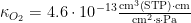
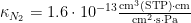
Key Thermal Constants
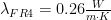
Figure 5 shows some of the constants used in the analysis to follow.

Figure 5: Key Thermal Constants.
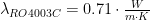
Thermal Resistance of the Silicon Die
The transistors on the IC dissipate power. Integrated circuits place their power dissipating elements on one side of a slab of silicon. This power must pass through the silicon to an aluminum slug, which conducts the heat from the silicon to the top of the PCB. Figure 6 shows the calculations.
Figure 6: Thermal Resistance of the Silicon Die.
Thermal Resistance of the IC's Heat Slug
Figure 7 shows the calculations for the thermal resistance of the heat slug.

Figure 7: Thermal Resistance of the Heat Slug.
Thermal Resistance of the Copper Pad on Top PCB Layer
Figure 8 shows the calculations of the copper pad on the top of the PCB. The IC's heat slug sits on this copper pad.

Figure 8: Thermal Resistance of the Copper Pad on Top of the PCB.
Thermal Resistance of the PCB
The PCB thermal model is a composite of vias, laminate, and planes. I break this modeling down in the following subsections.
Thermal Resistance of the FR4 PCB Material
Figure 9 shows how I calculated the thermal resistance of the FR4 PCB material.

Figure 9: Thermal Resistance of FR4 Material in the PCB.
Thermal Resistance of a 20 mil Via
Figure 10 shows the calculations for the thermal resistance of a 20 mil via.
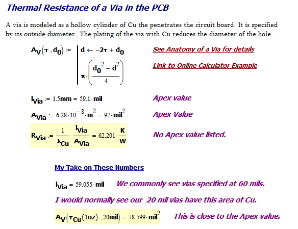
Figure 10: Formula for the Thermal Resistance of a Via.
Thermal Resistance of the PCB with 24 Vias
Figure 11 show the calculations for the thermal resistance of the overall PCB (i.e. FR4 material thermally in parallel with 24 vias). Observe that the vias have a combined thermal resistance of ~2.6 Ω, which is modeled as a parallel resistance to laminate's thermal resistance of ~58 Ω. Clearly, most of the heat moves through the vias.

Figure 11: Thermal Resistance of the Overall PCB.
Thermal Resistance of the PCB Bottom Copper Layer
Figure 12 shows how the thermal layer of the PCB's bottom copper layer is computed.

Figure 12: Thermal Resistance of the Bottom Copper Layer on the PCB.
Overall Thermal Resistance Calculation
Figure 13 shows the overall thermal resistance calculation. Observe that nearly 85% of the thermal resistance is in the PCB – without vias, this percentage and RTotal would have been much larger.

Figure 13: Total Thermal Resistance Calculation.
Conclusion
This was a good computation exercise. Let's review the results:
- This exercise presented a good example of a power-focused, analog design.
- This example used a heat sink – most digital designs do not include heat sinks.
- In applications without fans, getting the heat to the air is a big challenge.
- All the calculations were based on Equation 1, which is analogous to the formula for the resistance of an electrical conductor.
- The thermal resistance of the PCB dominates the overall thermal resistance
- Adding more copper to the PCB can help (e.g. 2 oz Cu planes), but this will make the PCB more difficult to solder and rework.
- The role of the via to the overall PCB thermal resistance is critical.
- You need to place as many vias as you can between the top and bottom layers.
- For high -power circuit boards, you may wish to use other laminate materials – their thermal resistance varies quite a bit
- FR4 is the cheapest laminate you can find. Any others will cost more.
Save
Save
Save
Save
Save
Save
Save


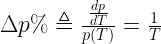
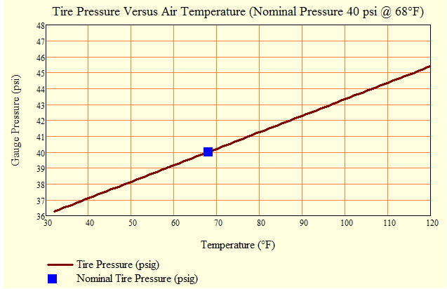
 is the percentage tire pressure change with temperature.