AC Backup Power Using A Simulated Sine Wave

Quote of the Day

Whenever you want to marry someone, go have lunch with his ex-wife.

- Shelly Winter


Introduction

Figure 1: Typical AC Signal At Wall Outlet.

Figure 1: Typical AC Signal At Wall Outlet (Source). The flat-top distortion is common – especially when many loads are switching power supplies.

A customer today requested an AC-output Uninterruptible Power Source (UPS) for our indoor Optical Network Termination (ONT) products. Product Management asked us to consider this unit from CyberPower. This unit, like most other AC-output UPS hardware, does not generate an actual sine wave output like the local power utility (Figure 1 – sine waves are what comes out of an AC outlet). Instead, it generates an output that is often referred to as a simulated sine wave (also known as a pseudo-sine wave, quasi-sine wave, modified sine wave, or Pulse-Width Modulated [PWM]). I thought it would be useful to look at the mathematics behind this type of output.

This backup power unit converts the DC voltage from the battery into a simulated sine wave that will imitate the behavior of a real sine wave for most loads. A pure sine wave inverter can be used in a lot of different ways so are worth looking into. A device that performs this operation is called an inverter. You might wonder why the backup power folks chose to put out a simulated sine wave rather than a true sine wave. Like most things in the engineering, the issue is one of cost. Another option one could look into is the Switch Mode Power Supply (SMPS). This is more cost-effective compared to a pure sine-wave inverter. You could find clear instructions that will assist you in troubleshooting switch mode power supplies at a faster rate on many websites.

Generating a pure sine wave is relatively expensive when compared to generating an approximation. For an example of a circuit for generating a bipolar (i.e. both positive and negative voltage levels) PWM output, see the Wikipedia. In my experience, the simulated sine wave works almost as well as a real sine wave for most applications. I have had a couple of instances that involve radio receivers where the simulated sine wave did not work well. In each case, the audio output was contaminated with noise that would not have existed with a real sine wave. I discuss the inverter that caused these issues in Appendix A. Other than those two cases, I have been able to successfully power everything from lights to computers using a simulated sine wave.

Background

Calling the output of this UPS a "simulated sine wave" is a bit of a stretch. The power waveform from an outlet is a sine wave (purple waveform in Figure 2). Observe that the "simulated sine wave" (reddish-brown waveform in Figure 2) does not look like a sine wave at all -- it is a form of pulse-width modulation. As is shown in Figure 2, the power supply output has only three output levels: +VA, 0 V, and -VA, where VA is amplitude of pulse-width modulation. Notice also that three time values are shown in Figure 2:

  • TH: the time during each period that the voltage output stays at VA
  • TL: the time during each period that the voltage output stays at -VA
  • T: the period of the signal

For the simulated sine wave to have zero DC level like that of the utilities' AC waveform, TH= TL. We will define the duty cycle to be \displaystyle D\triangleq {}^{\left( {{T}_{H}}+{{T}_{L}} \right)}\!\!\diagup\!\!{}_{T}\;.

Figure 1: Sine Wave Versus Simulated sine Wave.

Figure 2: Sine Wave Versus Simulated Sine Wave.

These backup units work by creating a pulse-width modulated output that has:

  • an amplitude comparable to the amplitude of a standard AC sine wave VA
  • an RMS value (VRMS) that is comparable to a standard AC sine wave
  • the same period as the standard AC sine wave (60 Hz in North America)

We will use a bit of mathematics to derive the relationship between VA, D, and VRMS.

Analysis

Requirements

Most AC-input powered equipment will work if they are presented with a simulated sine wave voltage waveform that has the same:

  • VA as the utility power sine wave
  • VRMS as the utility power sine wave
  • T as the utility power sine wave

We will derive expressions that will allow us to determine the required VA and VRMS values in terms of the nominal power line voltage and the duty cycle.

Derivation

Voltage Amplitude

Determining the required voltage amplitude is the easy. In the US, the nominal AC voltage at the power meter is set by ANSI C84.1-2011 at 120 V (RMS). The amplitude of a sinusoid is related to its RMS value by Equation 1.

Eq. 1 \displaystyle {{V}_{A}}=\sqrt{2}\cdot {{V}_{RMS}}=\sqrt{2}\cdot 120\text{ V=170 V}

So we should see our inverter putting out a voltage with an amplitude around 170 V.

RMS Voltage

Equation 2 shows how we can derive the relationship between VA, D, and VRMS.

Eq. 2 \displaystyle {{V}_{RMS}}=\sqrt{\frac{1}{T}\cdot \int\limits_{0}^{T}{V{{(t)}^{2}}\cdot dt}} Definition of RMS voltage
\displaystyle {{V}_{RMS}}=\sqrt{\frac{1}{\frac{T}{2}}\cdot \int\limits_{0}^{T/2}{V{{(t)}^{2}}\cdot dt}} Positive and negative pulses are symmetrical, so I will just integrate over half a period
\displaystyle {{V}_{RMS}}=\sqrt{\frac{1}{\frac{T}{2}}\cdot \int\limits_{T/4-D\cdot T/4}^{T/4+D\cdot T/4}{V_{A}^{2}\cdot dt}} The function is a constant during the on-portion of the duty cycle, zero otherwise
\displaystyle {{V}_{RMS}}=\sqrt{\frac{2}{T}\cdot V_{A}^{2}\cdot D\cdot \frac{T}{2}}=\sqrt{D}\cdot {{V}_{A}} Evaluate the integral
\displaystyle D={{\left( \frac{{{V}_{RMS}}}{{{V}_{A}}} \right)}^{2}}={{\left( \frac{1}{\sqrt{2}} \right)}^{2}}=\frac{1}{2} Compute D for a North American power system

This means that an inverter that generates a simulated sine wave with 170 V amplitude and a duty cycle of 50% will provide the same peak voltage amplitude and RMS voltage as is delivered from a North American wall outlet. For many applications, that is good enough.

Real UPS Output Example

Lab Note: My oscilloscope did not want to display the whole waveform on the screen, so I ended up running the output through a resistor divider that reduced its level by a factor of 33.8. This division factor allowed me to display everything with a minimum of fuss. So all voltages you see going forward will need to be multiplied by 33.8 to get their actual value.

Let's take a detailed look at the output voltage from a CyberPower CP550HG, which is a commonly used backup unit for PCs. Figure 3 shows an oscilloscope screenshot of the unloaded output from the CP550HG. I was lazy today and did not do any analysis of my own on the signal -- I just let the oscilloscope compute things like RMS voltage and period.

Figure 2: Oscilloscope Screenshot of Unloaded CP550HG Output.

Figure 3: Oscilloscope Screenshot of Unloaded CP550HG Output.

The key characteristics from this plot are:

  • Duty cycle of 49% (50% target)
  • Frequency of 60.770 Hz (60 Hz target)
  • Peak amplitude of 181 V = 33.8·10.7V/2 (170V target)
  • RMS output voltage of 125.2 V = 33.8·3.704 V (120 V target)

The numbers measured are all within the range I would have expected for this unit. Since these are numbers were measured with zero load, I would expect them to be a bit high and they are.

See Appendix A for the data I measured from an inverter I use to run my computer when I am in my car. This is a very cheap unit and its numbers are a bit different because their design goals were different.

Conclusion

I was able to derive the amplitude and duty cycle required for a simulated sine wave inverter to behave similarly to a North American 120 V power waveform and I verified this derivation with an actual test case from the lab. The values I measured were all as I would have expected.

Appendix A

Here is the Black and Decker inverter I use in my car (Figure 4). Overall, it has worked well for me over the past few years. However, it did corrupt the audio output from a couple of radios that I was trying out.

Figure 3: Black and Decker 400 W Inverter.

Figure 4: Black and Decker 400 W Inverter.

Here is a plot of its output (Figure 5).

Figure 4: Output From Black and Decker Inverter.

Figure 5: Output From Black and Decker Inverter.

It has a lower peak voltage than the CyberPower. They compensate for this by making the duty cycle longer, which increases the RMS voltage. This is the unit that has caused me trouble powering some radio gear.

I would summarize its characteristics as follows.

  • Duty cycle of 80%
  • Frequency of 59.6 Hz
  • Peak amplitude of 136.9 V
  • RMS voltage of 117.6 V

Since this unit does not have the same peak voltage as a utility sine wave, I would expect it may have some issues driving some types of loads and I have seen issues (mentioned above). They probably made the decision to reduce the output voltage because generating higher voltages costs more than generating lower voltages -- and cost drives everything in consumer products.

Posted in Electronics | 5 Comments

Great discussion of Saturn's Polar Hexagon

Quote of the Day

Limited funds are a blessing, not a curse. Nothing encourages creative thinking in quite the same way.

— L. Yau


Figure 1: Saturn's Hexagon as seen from Cassini Satellite.

Figure 1: Saturn's Hexagon as seen from Cassini Satellite. (Source)

This particular post discusses a very interesting laboratory experiment that illustrates how the hexagonal region at Saturn's pole may form.

Great discussion of Saturn's Polar Hexagon

Posted in Astronomy | Tagged , | Comments Off on Great discussion of Saturn's Polar Hexagon

Age Distribution of US Health Care Expenditures

Quote of the Day

The beginnings and endings of all human undertakings are untidy.

- John Galsworthy


Figure 1: Health Care Expenditure Percentage By Age Group.

Figure 1: Health Care Expenditure Percentage By Age Group.

I have been wondering why US health care costs are so high. I just read this report that claims that the US spends a far greater percentage of its health care dollars on the elderly than other countries. Increasing medical costs are common for the elderly because as we get older, we can develop various age-related illnesses. It's totally natural. When we get to a certain age, these illnesses can take over our lives. We might need to look for help from a Lynchburg home care agency or even try and find a more permanent place of residence that can provide assistance. Care homes are a popular choice for many of the elderly as they receive around-the-clock care and are able to enjoy the social elements that come with living with others in a similar situation to them. Many of us also choose to take out life insurance policies to cover the cost of any medical bills that may need to be paid after we pass. Life insurance policies and payments can vary, and you can click here to discover quotes if you need life insurance for yourself. But I always wondered if healthcare for the elderly is essential, why is it so expensive? I decided to plot the data from the report myself to make viewing the data a bit easier -- see Figure 1. The expenditures are normalized to the costs for people in the 50 to 64 year old age range (arbitrarily given a value of 1 unit). Here is what the chart tells me:

  • For citizens less than 65 years old, the distribution of US health care spending is not markedly different from other countries.
  • The US, Canada, and UK seem to be doing something distinctly different for their elderly than the other nations in the study, with a comparison between the Kew Gardens Aged Care and other care clinics able to be drawn.
  • The US expense distribution is markedly different than all other countries for people 65 year old and older.

For those who think that the problem is the percentage of old people in the US, remember that Japan has the oldest population in the world, yet their health care expense distribution is much flatter than that of the US. In actual fact, the US has favorable demographics compared to other nations in the study, whether that be for people who would need to access pharmacy services (such as these: https://southwestcare.org/services/support-services/pharmacy-services/) or other resources! Whilst there is no doubt we have some great services in this country when it comes to medical needs, it is interesting to see it through comparisons to other nations.

Save

Posted in Financial | 4 Comments

Great Article on Recreating Shackleton's Whiskey

Quote of the Day

Play is the only way the highest intelligence of humankind can unfold.

— Joseph Chilton Pearce


Figure 1: Shackleton's Whiskey Bottle. (Source)

Figure 1: One of Shackleton's Whiskey Bottle. (Source)

While I am not a drinker, I do admire the impressive technology that Scottish distillers used to duplicate the lost recipe for Shackleton's whiskey.  They were even able to identify where the peat used in its formulation came from.

Great Article on Recreating Shackleton's Whiskey

Save

Posted in General Science | Tagged | Comments Off on Great Article on Recreating Shackleton's Whiskey

Fond Memories of Fast-Moving Milk Bottles and Toy Boats

Quote of the Day

Write freely and as rapidly as possible and throw the whole thing on paper. Never correct or rewrite until the whole thing is down. Rewrite in process is usually found to be an excuse for not going on.

— John Steinbeck


Figure 1: Machine Filling Milk Bottles. (Source)

Figure 1: Machine Filling Milk Bottles. (Source)

Last night, I was watching a show on the Science Channel called How It's Made. This episode reminded me of an old movie I was shown in elementary school that started my interest in science and math. The message here is that you never know what will stimulate the interest of a child.

Last night on "How It's Made" they were showing machines filling bottles with a beverage. This show stimulated my memories from first-grade when I was shown a 16mm movie about how milk came to our door every morning. I still can remember almost every detail of this movie. The story started with a cow eating grass and ended with a bottle of milk on a kitchen table. What really caught my eye was the filling of the milk bottles by machines. It seemed like magic the way the bottles were put into a fast-moving row, filled while moving in a circle, and then capped. I became driven to learn how those machines worked and to build my own machines. I began my quest by asking Santa for an erector set. Things just grew from there.

Back in those days, every house in the town of Osseo had a small box that a milkman would fill with glass bottles of milk. The picture below is very similar to the milk box that my family had.

As the oldest of five children, one of my jobs was to move the milk from the box to the refrigerator. Seeing the magic that brought milk to our door made the mundane seem really interesting.

Youtube has many videos showing bottles being filled. I cannot find the original movie that I saw, but the video embedded below is similar in content to the bottle-filling sequence from the movie I saw originally.

While I am on the subject of children's videos, I noticed that Paddle to the Sea is also on Youtube. This is a very cute video that also made an impression on me. I actually tried to carve my own little wooden boat after seeing this movie back in second-grade.

Posted in General Science, Osseo, Personal | 1 Comment

The Joys of Electrostatic Discharge

Quote of the Day

The only people with whom you should try to get even are those who have helped you.

— John E. Southard


I had to laugh at this Youtube video this morning. This poor guy shows you exactly how NOT to handle hardware during ElectroStatic Discharge (ESD) tests.

Posted in Electronics | 3 Comments

Parabolas and Avalanche Photodiodes

Quote of the Day

You have to perform at a consistently higher level than others. That's the mark of a true professional.

— Joe Paterno


Introduction

Figure 1: Typical Avalanche Photodidoe.

Figure 1: Typical Avalanche Photodiode. (Source)

During a meeting recently, a vendor was discussing the need for performing production calibration testing that required fitting a parabola to the data from an optical sensor called an Avalanche PhotoDiode (APD) (Figure 1). I recalled this comment while reviewing a test report this morning where I saw a parabola appear in an APD test report from an optical physicist in my group. I realized that our physicist and this vendor were working in related areas. It was an excellent test report that covered both the theoretical and experimental aspects of the subject. It also seemed like a good topic for this blog.

I thought this was a good example of a common situation in electronics:

  • You need to determine a physical parameter (e.g. average optical power) that is a function of some electrical parameter (e.g. voltage across a resistor).
  • The parameter is a nonlinear function of the electrical parameter -- in this case, the nonlinear function is a parabola.
  • Each component will have a slightly different nonlinear function that must be determined during the production testing for each part.
  • You want to minimize the amount of production data you must gather because the cost of gathering data increases with the amount of data.

This post will provide a brief description of how an APD is used in a optical receiver circuit and how we can measure the average optical power received by the APD.

Background

Optical Networks

My group builds Optical Network Units for GPON systems. The ONUs are mounted on the sides of homes and they contain both optical transmitters (i.e. lasers) and receivers (i.e. APDs). The APDs detect the light pulses on the fiber that convey information to the home. APDs are capable of detecting very small changes in light level -- in fact, they can even count individual photons when the used in the correct circuit. In this particular case, we want to measure average optical power and not instantaneous power.

The whole concept of using avalanche phenomena to create very sensitive detectors is an old one. APDs are very similar in concept to the Photomultiplier Tube (PMT). Geiger counters also use similar technology.

APD Background

For our work here, I am going to treat the APD as a mathematical object -- no circuit details. These details are not need to understand how we can measure average optical power using a photodiode. For our purposes here, there are three things we need to know about APDs:

  • They convert optical power into current.
  • The conversion factor between optical power and current is a function of the voltage applied to the APD.
  • The conversion factor is a highly nonlinear function of the voltage applied to the APD.

Equation 1 is the key equation showing the relationship between optical power and APD current.

Eq. 1 {{I}_{APD}}=M({{V}_{APD}})\cdot \mathscr{R} \cdot {{P}_{O}}

where

  • IAPD is the current through the APD.
  • VAPD is the voltage across the APD. This voltage is set during production to provide the desired level of amplification.
  • M(VAPD) is an adjustable gain (i.e. multiplication) factor. This is useful because we need to ensure that current from the APD is kept within the range of values that our electronics can measure.
  • \mathscr{R} is the responsivity of the photodiode. It is a conversion factor from optical power (Watts) into current (Amperes).

The multiplication factor, M(VAPD), is described by Miller's formula, which I state in Equation 2.

Eq. 2 M\left( {{V}_{APD}} \right)=\frac{1}{1-{{\left( \frac{{{V}_{APD}}}{{{V}_{B}}} \right)}^{n}}}

where

  • VB is the breakdown voltage of the APD. This is a critical parameter for all APDs.
  • n is a parameter that varies with the design of the specific device. We will assume n=1 for our work here.

During manufacturing, we adjust VAPD to achieve the desired gain. The setting of the gain is always a "Goldilock's Problem" -- the gain must be high-enough so that you can detect the minimum signal level you expect to encounter, but not so high that you saturate your detector with the maximum signal level you expect to encounter.

Current Mirror

The Wikipedia has a good working definition of a current mirror.

A current mirror is a circuit designed to copy a current through one active device by controlling the current in another active device of a circuit, keeping the output current constant regardless of loading.

In the case here, our current mirror actually makes a duplicate of 1/5 of the APD current. This scaling is useful because the APD current range is so wide that it is difficult to measure accurately without reducing its range.

Analysis

Schematic

Figure 2 is a simplified schematic of the receiver circuit. The circuit here is based on one in a Maxim application note. There are different ways of implementing receivers, but this is a reasonable one.

Figure 1: Simplified Schematic of the Optical

Figure 2: Simplified Schematic of the Optical

Figure 2 deserves a few comments:

  • VOut is connected to the input of an A/D converter.

    The A/D converters have a limited range of voltages that they can convert. A typical range would be 0 V - 2.00 V. The current in the APD will increase as the APD receives more optical power.

  • CBypass is used to filter the APD current.

    For optical diagnostics, we are interested in the average optical power at the ONT. To measure the average optical power, we need to filter out the variations due to short-term variations about the average power due to changes in bit values (zero or one).

  • We measure the APD current by measuring the voltage across ROut.

    The use of the current mirror eliminates the need to make a direct measurement of the APD current.

Derivation of Optical Power Versus Output Voltage

After a bit of algebra, we can derive the parabolic relationship between optical power and VOut, which is shown in Equation 3. Observe that Equation 3 is a quadratic with no constant term.

Eq. 3 {{P}_{Optical}}=\frac{1}{{{K}_{A}}}\cdot \left( \frac{{{R}_{Sense}}}{\mathscr{R}\cdot R_{Out}^{2}\cdot {{V}_{B}}\cdot K_{M}^{2}}\cdot V_{Out}^{2}+\left( \frac{{{R}_{Out}}\cdot {{V}_{B}}}{\mathscr{R}\cdot R_{Out}^{2}\cdot {{V}_{B}}\cdot {{K}_{M}}}-\frac{{{R}_{Out}}\cdot {{V}_{App}}}{\mathscr{R}\cdot R_{Out}^{2}\cdot {{V}_{B}}\cdot {{K}_{M}}} \right)\cdot {{V}_{Out}} \right)

where

  • KM is the mirror current scaling. We are using 1/5 in this circuit.
  • KA is the relationship between the low-frequency component and total current values of the APD current. We will assume this value to be 1 in this case. In this application, the actual value is not important. It is a constant.
  • RSense is a the resistor we use to sense the APD current value.
  • VAPP is the supply voltage used to drive the APD bias voltage, which is constant.

The details of the derivation are shown in Figure 3, which is a screenshot of a part of a Mathcad worksheet. Note that I did perform some minor algebraic manipulation of the Mathcad output to obtain Equation 3, which is a form that is a bit more useful to me.

Figure 2: Derivation of Optical Power Versus Output Voltage.

Figure 3: Derivation of Optical Power Versus Output Voltage.

Comparison with Empirical Results

In production, we will not be measuring all the individual parameters shown in Equation 3. Instead, we use the parabolic form derived above and determine the associated polynomial coefficients by fitting production calibration data to Equation 4. This approach is simpler and does not require gathering large amounts of data.

Eq. 4 {{P}_{Optical}}={{K}_{2}}\cdot V_{Out}^{2}+{{K}_{1}}\cdot {{V}_{Out}}

where

  • K2 and K1 are coefficients to be determined by curve fitting.

Observe how Equation 4 always passes through the origin. In actual use, we may choose to use a quadratic equation that includes a constant term (hence, three coefficients instead of two) because analog electronic parts always have DC offsets present that may be large enough that they must be compensated for.

Figure 4 shows how the empirical data compares to the parabolic model fitted to the data. The fit is very good.

Figure 3: Comparison of Empirical Data to Parabola Fitted to Data.

Figure 4: Comparison of Empirical Data to Parabola Fitted to Data.

In Figure 4, I used a large amount of data in the fitment process. In an actual manufacturing environment, every data point measured costs money. This model is for a parabola that passes through the origin. At a minimum, this means that only two more data points are needed to determine the required parabola. However, real measurements are always contaminated with noise and gathering additional data points can minimize the impact of this noise. There is a tradeoff that must be made between accuracy and cost.

Conclusion

This post shows a common sequence of mathematical modeling operations for an engineer:

  • Develop a formula template based on theory.
  • Perform lab experiments to verify the model.
  • Verify the data gathered fits the formula template that was developed.
  • Develop an efficient procedure for performing curve fitting in a production environment.

Save

Save

Save

Save

Save

Save

Save

Save

Save

Save

Save

Save

Posted in Electronics | Comments Off on Parabolas and Avalanche Photodiodes

Battery Failure Rates and Continuously-Compounded Interest

Quote of the Day

The man who does not read good books has no advantage over the man who cannot read them.

— Mark Twain


Introduction

7.2 A-hr Sealed Lead Acid Battery.

Figure 1: A Common Sealed Lead Acid Battery.

While performing some routine reliability analysis, I noticed that there is a similarity between battery aging and continuously-compounded interest calculations. I had not noticed this similarity before, and I thought I would document it here.

Figure 1 shows a common lead-acid battery. This chemistry is my focus in this post. Other chemistries will behave similarly, but the constants involved will differ. I will be assuming that the failure rate of the battery is described by the Arrhenius equation.

Background

To understand this post, we need to establish a bit of knowledge in two areas:

  • Chemical Reaction Rates and the Arrhenius Equation
  • Continuously Compounded Interest

Chemical Reaction Rates and the Arrhenius Equation

Batteries are chemical machines and their performance is predictable using the mathematics of chemical kinetics. For our purposes here, the key equation is the Arrhenius Equation, which I state in Equation 1.

Eq. 1 \displaystyle k=A\cdot {{e}^{-\frac{{{E}_{a}}}{R\cdot T}}}

where

  • A is a reaction-dependent constant.

    My work here will involve only relative values, which means that the exact value of A will not be important.

  • T is the absolute temperature.

    A common calculation error is to work in celsius and not Kelvin. Make sure that all your battery work is in Kelvin.

  • Ea is the activation energy.

    The primary corrosion reaction has an activation energy of about 50 kilo-Joules (kJ) per mole (reference).

  • R is the universal gas constant.

The Wikipedia has a very good article on the Arrhenius equation. I have also reviewed the Arrhenius equation in earlier post, and I will assume those in need of further review will venture there.

Continuously Compounded Interest

The Wikipedia provides some good background on continuously compounded interest. I will review the mathematics behind continuous compounding briefly here.

Equation 2 shows the basic compound interest formula.

Eq. 2 \displaystyle A=A_0 \cdot {{\left( 1+\frac{r}{n} \right)}^{n \cdot t}}

where

  • A is the final value of the investment (principal and interest)
  • A0 is the principal amount (initial investment)
  • r is the annual nominal interest rate
  • n is number of times the interest is compounded per year
  • t is number of years the investment receives interest payments

Assume that we want to compute the interest paid after one year (t = 1) to an account where the interest is compounded an infinite number of times (n = ?). Equation 3 shows the basic steps in the derivation.

Eq. 3 {{A}_{\infty }}=\underset{n\to \infty }{\mathop{\lim }}\,\ {{A}_{0}}\cdot {{\left( 1+\frac{r}{n} \right)}^{n\cdot t}}={{A}_{0}}\cdot {{e}^{r\cdot t}}

where

  • A? is the final value of the investment after infinitely many compounding cycles.

Assume we are interested in the amount of time required to double our investment assuming continuous compounding. Equation 4 illustrates that computation.

Eq. 4 \displaystyle 2\cdot A=A\cdot {{e}^{r\cdot t}}\Rightarrow t=\frac{\ln (2)}{r}

This equation is related to the famous "Rule of 72", which makes calculations of investment doubling time simple enough to do in your head (see here and here). It turns out that Equation 4 is also useful in computing the temperature increase required to halve the life of a battery.

Analysis

Battery Longevity's Relationship to Chemical Reaction Rates

The battery's longevity is determined by the speed of the corrosion reaction -- a faster corrosion reaction will corrode the battery faster and bring its demise sooner. No wonder why the concept of passivation is essential for metal. Not everyone is going to understand this topic in particular, but through companies such as astropak, you can learn even more about what the process of passivation involves. You learn something new everyday.
We can derive the impact of this faster corrosion reaction on the battery's lifetime by making a couple of assumptions:

    • The battery is considered failed when its capacity has been reduced below the level needed to provide adequate backup capacity.

      In the telcom industry, we normally consider a battery to have failed when its backup capacity is reduced to 80% of its initial value (see Telecordia's GR-909 for details)

    • Corrosion will gradually reduce the battery's capacity.

      The effects of corrosion are measurable in terms of battery impedance. UPS hardware usually incorporates some form of load test in order to determine if the battery's capacity has fallen a desired level.

Equation 5 shows that the battery lifetime will degrade exponentially with increasing temperature.

Eq. 5 D=\tau \cdot A\cdot {{e}^{-\frac{{{E}_{a}}}{R\cdot {{T}_{0}}}}}
{{D}_{0}}={{\tau }_{0}}\cdot A\cdot {{e}^{-\frac{{{E}_{a}}}{R\cdot {{T}_{0}}}}}
\tau =\frac{{{D}_{0}}}{A}\cdot {{e}^{\frac{{{E}_{a}}}{R\cdot T}}}={{\tau }_{0}}\cdot {{e}^{-\frac{{{E}_{a}}}{R\cdot {{T}_{0}}}}}\cdot {{e}^{\frac{{{E}_{a}}}{R\cdot T}}}
\tau ={{\tau }_{0}}\cdot {{e}^{-\frac{{{E}_{a}}}{R\cdot T\cdot {{T}_{0}}}\cdot \left( T-{{T}_{0}} \right)}}
\tau ={{\tau }_{0}}\cdot {{e}^{-\frac{{{E}_{a}}}{R\cdot T\cdot {{T}_{0}}}\cdot \Delta T}}

where

  • ? is the battery's lifetime at a temperature of T.
  • ?0 is the battery's lifetime at a temperature of T0.
  • T is the battery temperature for which we require an estimated lifetime.
  • ?T=T-T0.
  • D0 is the total amount of the corrosion chemical reaction required to degrade the battery to failure.
  • D is the total amount of the corrosion chemical reaction for a battery at a temperature of T for a time ?.

Unfortunately, Equation 5 contains two unknowns (i.e. ?T and T). We cannot directly solve Equation 5 without making an approximation. If we are only interested in temperatures near our reference temperature (T0), we can say that {{T}_{1}}\approx {{T}_{0}}\Rightarrow {{T}_{1}}\cdot {{T}_{0}}\approx T_{0}^{2} . Equation 6 gives us a useful approximation for the battery's lifetime at a temperature near the battery's reference temperature.

Eq. 6 \tau \approx {{\tau }_{0}}\cdot {{e}^{-\frac{{{E}_{a}}}{R\cdot T_{0}^{2}}\cdot \Delta T}}

Observe that Equation 6 is similar in form to Equation 3:

  • ?T in Equation 5 corresponds to t in Equation 3.
  • {{\tau }_{0}} in Equation 5 corresponds to A0 in Equation 3.
  • {{\tau }} in Equation 5 corresponds to A in Equation 3.
  • E_a / \left( R \cdot T0^2 \right) in Equation 5 corresponds to r in Equation 3.
  • ?T is the increase in temperature needed to halve the lifetime of the battery.

Given these correspondences, we can state that the temperature difference required to halve the battery lifetime is given by Equation 7, which is just Equation 3 with the listed substitutions.

Eq. 7 \frac{1}{2}\cdot {{\tau }_{0}}={{\tau }_{0}}\cdot {{e}^{-\frac{{{E}_{a}}}{R\cdot T_{_{0}}^{2}}\cdot \Delta T}}\Rightarrow \Delta T=\frac{\ln \left( 2 \right)}{\frac{{{E}_{a}}}{R\cdot T_{0}^{2}}}

Figure 2 provides an example for how the lifetime halving temperature for a typical lead-acid battery is computed.

Figure 1: Temperature Increase that Halves Battery Lifetime.

Figure 2: Temperature Increase that Halves Battery Lifetime.

The calculation in Figure 1 confirms that 10 °C value given here.

Conclusion

I found it interesting that a relationship I have used for years in financial analysis is also useful in battery life calculations. There is something almost magical about the way similar mathematics occurs in very diverse areas.

Save

Save

Posted in Batteries, Electronics | 1 Comment

Lead Acid Battery Life Math

Quote of the Day

The key to effective goal-setting is being realistic about what you can accomplish.

— Andrea Woroch


Introduction

7.2 A-hr Sealed Lead Acid Battery.

Figure 1: A Typical 7.2 A-hr Sealed Lead Acid Battery.

It is difficult to dig trenches for fiber optic cable in many parts of the US and Canada during the winter. Thus, winter is the time of year when telecommunications companies do their planning for fiber optic deployments during the following spring, summer, and fall. This planning time is when the service providers see the large amount of money they spend on replacing bad lead-acid batteries, and they start to ask what they can do to reduce the failure rates of these batteries. These inquiries are about as predictable as the arrival of Christmas. Today, I received a more detailed question than I usually do and I thought my answer was worth documenting for a wider audience.

Background

Battery Construction

Figure 2 shows a video that does a nice job showing how batteries are built.

Figure 2: Good Video Briefing on Battery Construction.

Battery Life Reduction With Increasing Temperature

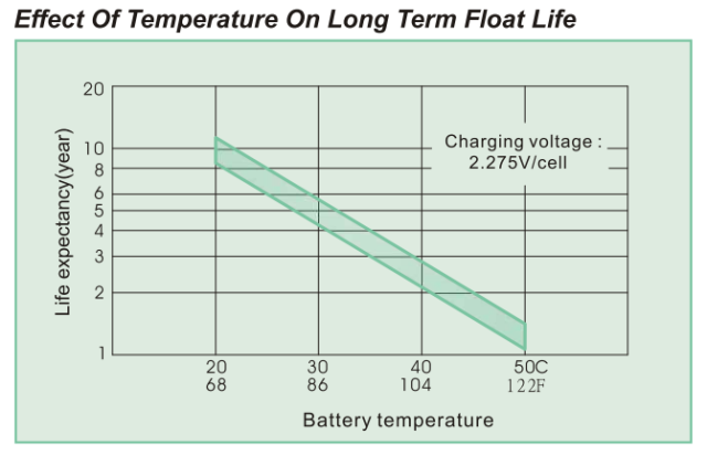
Today, I was shown this specification and asked to explain how battery life can change so much with temperature. Figure 3 shows the battery life graph that was the focus of this discussion.

Figure 1: Battery Life Versus Temperature.

Figure 3: Battery Life Versus Temperature.

Figure 3 is a semi-log plot of the projected life of a 7.2 A-hr, Valve-Regulated Lead Acid (VRLA) battery versus temperature. Note that a range of battery lifetimes is given by this plot. This makes sense because battery lifetime will vary from unit-to-unit. Battery customers need to understand that battery life is not guaranteed -- you lifetime will vary based on the particular unit you have and how you treat it.

Failure Mechanism

Battery used in backup applications spend most of their lives at a float voltage. The main mechanism of failure in float applications is corrosion. Since I am not an electrochemist, I will simply quote a paper by a student of a battery expert:

The primary unavoidable aging effect is corrosion of the positive grid, composed initially of metallic PbO2, and is probably the most important factor for calendar life. This effect is also called grid growth because the electrode physically expands. [Wager] gives details on how the design of VRLA batteries can impact this fault mode, and on the chemistry of the process. In a nutshell, although we say that the positive electrode is composed of PbO2, this lead dioxide forms a dense corrosion layer around the metallic lead in the positive electrode when fully charged. This layer shrinks and expands during discharge and charge, and as it becomes fixed in a state of permanent corrosion, the grid is said to be corroded.

This quote is from this paper. Appendix A has a good infographic on how corrosion occurs.

While lead-acid batteries are simple at a high-level, there are many complexities when you start looking at the details of how they operate and eventually die. For a very good look at the details of battery chemistry, see this paper.

Analysis

Failure Analogies to Self-Discharge

VRLA batteries in backup applications maintain their batteries at a float voltage level, usually between 13.6 V and 14.4 V. You often see batteries described as having a life of 300-500 discharges. But what does this mean with respect to a backup power application where the battery is rarely discharged? Batteries in backup applications do fail, usually by damage caused by corrosion and not by charge/discharge cycles. This corrosion is a chemical reaction similar to the reactions that cause self-discharge, which I discuss at length here.

Standard Reliability Model

Equation 1 show the model used by most VRLA battery vendors. Unfortunately, the vendors use different values for T0 and T1, which means that you have to be careful about making direct comparisons.

Eq. 1 L={{L}_{0}}\cdot {{\left( \frac{1}{2} \right)}^{\frac{T-{{T}_{0}}}{{{T}_{1}}}}}

where

  • L_0 is the expected device lifetime at the reference temperature T_0.
  • T_0 is the temperature at which the device has lifetime L_0.
  • T_1 is the temperature increase required to halve the expected lifetime of the device.
  • T is the actual operating temperature. Note that few batteries spend their entire lives at a constant temperature. I will address the variable temperature case in a later post.

Equation 1 is actually an approximation based on the Arrhenius equation. I review the details of this approximation here.

Model Characteristics For Figure 2

Equation 1 can be used to generate the curve of Figure 1. The required parameters are:

  • L_0 = 10 years (the graph actually shows a small range -- this reflects the natural variability seen between units).
  • T_0 = 20 °C.
  • T_1 = 10 °C.

I did not need to do any analysis to make this determination. The battery is rated to have a nominal life of 10 years at 20 °C and you can see that the life halves every 10 °C. You can read these values right off of the graph.

IEEE Approach

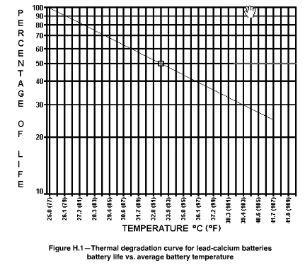
Note that Figure 3 describes a situation slightly different than that presented by the IEEE (Figure 4). IEEE Standard 450-2002 for lead-calcium alloy VRLA batteries sets T0 = 77 °F and T1 = 15 °F. Minor differences between models like this are not surprising -- batteries are all built slightly differently, and these difference will affect their expected lifetime.

Figure 2: IEEE Thermal Degradation Curve for Lead Calcium Batteries.

Figure 4: IEEE Thermal Degradation Curve for Lead Calcium Batteries.

People always seem surprised that lower temperatures mean longer battery life -- it is true. However, the capacity of the battery is reduced over its nominal value (i.e. Amp-hr capacity @ 77 °C). This means that customers in cold climates may need to have larger battery packs (i.e. higher capacity) to provide the backup time they need under cold conditions.

Conclusion

This is just a quick note to document some of the material I went through today. I do have anecdotal evidence in support of Equation 1. Our customers in hot climates (i.e. Texas) that use outdoor batteries see relatively short lifetimes. We also have customers in cold climates (i.e. northern Minnesota) who have had good battery performance for long past their nominal ratings.

Appendix A: Good Battery Sludge Generation Infographic.

Figure 5 shows a good infographic on how battery sludge builds up in a battery (Source).

Figure M: Infographic on Battery Sludge Generation.

Figure 5: Infographic on Battery Sludge Generation.

Save

Save

Save

Posted in Batteries, Electronics | 2 Comments

Battery Charge Capacity and Energy Math

Introduction

I am doing some requirements analysis work on backup power systems for GPON ONTs. As part of this work, I need to perform an evaluation of a number of batteries for charge capacity and energy. As part of this evaluation, I decided to write a Mathcad worksheet to perform the analysis. When I write an analysis routine, I usually test it using some data that has already been acquired and processed. In this case, I grabbed some data from the web and used this data to test my worksheet. If you wish to look at the actual worksheet, you can download it here.

Background

I will be evaluating some lithium-ion batteries for charge capacity and energy as a function of the battery's discharge termination voltage (i.e. battery voltage at which discharge current is terminated). Not everyone is going to understand this topic in particular, but you can learn something new everyday such as the Avocet Battery Materials that go into lithium-ion batteries. However, the same approach can be used for any battery.

Reference Battery Data

I did some in depth analasys for my reference data on lithium-ion batteries and found some excellent data on this web site, which I will replicate here. The data is for a single-cell, lithium ion (LiCoO2) battery (type 18650). Like I mentioned before, there is a lot of excellent data on the web about this kind of battery.

Figure 1 shows data for this battery in the same format as I often receive from our lab when testing batteries. Basically, you use a current source to apply a fixed load on the battery. You then measure the variation in battery voltage versus time.

Figure 1: Battery Voltage Versus Discharge Current At Fixed Current Loads.

Figure 1: Battery Voltage Versus Discharge Current At Fixed Current Loads.

In addition to the raw test data, this web site also contains graphs of energy (Watt-hours) and charge capacity (amp-hours). Thus, I can compare my worksheet's results with those of the web site as check on my routine's correctness.

Analysis

Gather Battery Data

Using Figure 1 and Dagra, I converted the graph into numeric form. Figure 2 shows how this data appears in my Mathcad worksheet. Normally, I receive this data from the lab in the form of an Excel spreadsheet. Because I am looking for test data prior to doing my own tests, grabbing some test data from an exisiting graph is a good way to evaluate my Mathcad worksheet.

Figure 2: Captured Data in My Mathcad Worksheet.

Figure 2: Captured Data in My Mathcad Worksheet.

The arrays A, B, C, D, E, F each contain two columns of data (time and battery voltage) that corresponds to discharge currents 0.2 A, 0.5 A, 1.0 A, 2.0 A, 3.0 A, and 5.0 A, respectively.

Compute Battery Energy

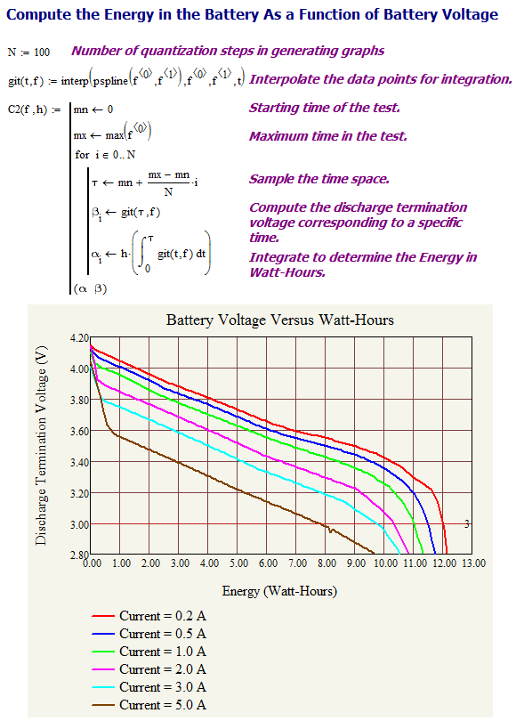
The energy extracted from a battery as we draw current from it is given by Equation 1, which assumes the discharge begins with a battery charged to 4.2 V. As we draw energy from the battery, its terminal voltage decreases. Equation 1 will be used to generate a plot of energy drawn versus battery voltage.

Eq. 1 E\left( v \right)=\int\limits_{0}^{\tau }{{{v}_{Battery}}\left( t \right)\cdot {{i}_{Battery}}\left( t \right)}\cdot dt

where

  • E(v) is the energy drawn from the battery as the terminal voltage has dropped to v [Watt-hours].
  • vBattery(t) is the battery voltage [V].
  • iBattery(t) is the current being drawn from the battery [A].
  • is the time at which vBattery=v [hours].

Figure 3 shows the Mathcad formulas I used to compute the battery energy and a plot of the data generated from this analysis.

Figure 3: Calculation of Battery Energy.

Figure 3: Calculation of Battery Energy.

Compute Battery Capacity

The calculation of the battery capacity is a bit simpler than the calculation of battery energy. The formula I used is shown in Equation 2.

Eq. 2 \displaystyle Q(v)=\int\limits_{0}^{\tau }{{{i}_{Battery}}}\left( t \right)\cdot dt

where

  • Q(v) is the charge drawn from the battery as the terminal voltage has dropped to v [Ampere-Hours].

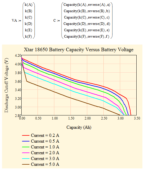
Figures 4 shows how the charge capacity calculation was setup. Note that while Equation 2 contains an integral, the use of a constant current source load means that we just need to compute the product of the current and time.

Figure 4: Formula Setup for Battery Capacity Calculation.

Figure 4: Formula Setup for Battery Capacity Calculation.

Figure 5 contains that graph of the charge capacity calculation results.

Figure 5: Capacity Calculation Results.

Figure 5: Capacity Calculation Results.

Conclusion

My worksheet generates very similar results to those posted on the reference web site. The only differences that I see between Figures 6 and 7 and the results my worksheet is generating are related to errors in grabbing the data off of the images -- there is always some error in that process.

At this point, I feel comfortable that my Mathcad routine is running properly and I can use this routine to process data being taken in my lab.

Figure 6: Vendor Measurements of Battery Capacity.

Figure 6: Vendor Measurements of Battery Capacity.

Figure 7: Vendor Data on Battery Energy.

Figure 7: Vendor Data on Battery Energy.

Posted in Batteries, Electronics | 4 Comments