
One of the engineers was sending this around today. I thought it was amazing.
One of the engineers was sending this around today. I thought it was amazing.
Quote of the Day
In any project, the important factor is your belief. Without belief, there can be no successful outcome.
— William James
My sons always tease me about my interest in space. In order to understand my interest in space, you need to understand what it was like being a boy during the 1960s. I had my own October Sky boyhood. I built rockets, read everything I could about space, built electronic circuits, and dreamt of someday being an engineer and space traveler. While the space traveler part didn't work out, I was fortunate in that I did everything else that I dreamt about it. I have met numerous engineers who are now in their 50s who had the same experiences.
I still read everything I can find about space. Recently, I was reading about Mars Science Laboratory (MSL) and noticed that it has a Radioisotope Thermoelectric Generator (RTG) for a power source. Figure 1 shows an artist's rendering of the MSL with two RTGs, which NASA refers to as the Radioisotope Power System (RPS).
.")
Figure 1: Mars Science Laboratory Rover with Radioisotope Power System (aka RTG-based Power System).
MSL's use of an RTG got me thinking about a physicist I sat next to on a flight years ago. He worked for Medtronic and had assisted in the development of a "nuclear battery" for use in a pacemaker. It was on that flight that I learned a little bit about RTGs. Let's see if we can use a bit of math to understand how an RTG works and how it is used on the MSL mission. As usual, I will be using Mathcad for the heavy lifting.
Referencing the Wikipedia, lets start with a definition of what an RTG is:
A radioisotope thermoelectric generator (RTG, RITEG) is an electrical generator that obtains its power from radioactive decay. In such a device, the heat released by the decay of a suitable radioactive material is converted into electricity by the Seebeck effect using an array of thermocouples.
Figure 1 (Source) shows a photograph of the RTG used on MSL, which is called the Multi-Mission RTG (MMRTG).

Figure 1: Photograph of MSL's MMRTG.
I saw the following statement in The Atlantic Magazine about the MMRTG:
The 43kg MMRTG is designed to produce 125 watts of electrical power at the start of the mission, falling to about 100W after 14 years. (NASA/Kim Shiflett)
Let's see if we can use this one statement to derive some information about the MSL's RTG.
A thermoelectric generator requires heat to produce electricity. Unfortunately, thermoelectric generators are notoriously inefficient. NASA has reported that their efficiency level is about 6.2%. This means that for every 1000 W put in, only ~62 W of electricity comes out. Since this generator is specified to put out 125 W, we need a heat source that produces 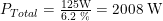
When a plutonium-238 atom decays, it emits an alpha particle with a decay energy of 5.593 Million Electron Volts (MEV). It is this decay energy is the source of heat (i.e. energy) that will be converted to electricity by thermocouples. This heat is enough to cause the Pu-238 to glow (see Figure 2, Source).

Figure 2: A Glowing Pu-238 RTG Element.
Radioactive decay versus time is usually modeled mathematically using the concept of half-life. Equation 1 shows how half-life is used to model decay.
| Eq. 1 |  |
where
To compute the power radiated by a sample of Pu-238, we need to determine the number of decays that occur per second. We can compute the number of decays per second by differentiating Equation 1, which I show in Equation 2.
| Eq. 2 |  |
Let's say we want to compute the amount of heat generated by a gram of Pu-238. We need to determine the number of Pu-238 atoms in a one gram sample and apply Equation 2, which tells us that Pu-238 generates 0.568 W/gm of heat. Figure 4 illustrates this calculation. We can use this number to estimate the amount of Pu-238 that we will need to generate 2 kW of thermal power.

Figure 4: Calculation of Heat Generated Per gm of Pu-238.
Since we know that we require 2 kW of thermal power and that Pu-238 generates 0.568 W/gm, we see that we need 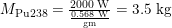
The quote from The Atlantic Magazine states that the electrical power available from the MMRTG drops to 100 W after 14 years. Let's assume that we have a fixed percentage of degradation year over year, which is similar to a compound interest problem. We can determine the percentage decline per year as shown in Equation 3.
| Eq. 3 |  |
So the output power is declining by 1.58% every year.
The amount of heat available from a radioactive source degrades every year because the amount of radioactive material reduces every year because of decay. We can compute this decline in thermal power as shown in Equation 4.
| Eq. 4 | |
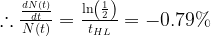 |
So thermal power declines by 0.79% every year, which is about half of the electrical power drop reported by NASA. However, the thermocouples also degrade in performance every year. So the 1.58% degradation rate is composed of two parts: (1) the reduction in available thermal power due to radioactive decay, and (2) the reduction in thermocouple conversion efficiency over time.
It turns out that there is data from Voyager on RTG power reduction. Over a 33 year period, Voyager has seen its available electrical power decline to 67% of its initial value, though its available thermal power has only declined by 83.4%. This means that Voyager has seen a decline in electrical power generation of 1.7% per year while its thermal power has degraded by 0.79% per year. So that 1.6% degradation expected for the MMRTG by NASA seems reasonable.
I was able to calculate some important characteristics of NASA's power system for the Mars Science Laboratory. I could see problems like this being good ones for calculus students to sharpen their skills on.
There are folks looking at how to improve the efficiency of nuclear batteries (example).
One of my sons asked me if I could work through a PageRank calculation example a couple of different ways (algebraic and iterative). It was an interesting exercise and I thought it would be worth documenting here. I used Mathcad for both my algebraic and iterative solutions.
Wikipedia has an excellent definition of the PageRank algorithm, which I will quote here.
PageRank is a link analysis algorithm, named after Larry Page[1] and used by the Google Internet search engine, that assigns a numerical weighting to each element of a hyperlinked set of documents, such as the World Wide Web, with the purpose of "measuring" its relative importance within the set.
Businesses and individuals who want their site to rank more highly in Google's search results could look at the services of a Digital Marketing Company to help boost their position.
PageRank is computed using a relatively simple function (see Equation 1), but a number of web-based examples treat the weighting of inbound links from sites external to a particular group of pages as a special case. I did not see any explicit calculation examples, so I thought I would include this calculation here. You'll more than definitely want to take this calculation into consideration if you're wanting to learn to how to build a website as well as wishing to attract traffic to your new site. Speaking of which, are you in the process of designing a new website? Whether you are a business or a blogger, running a website ensures that people that are interested in your products or services can learn about them with ease. So, have a web designing agency like The Web Designer Cardiff (click here) to have one made for you professionally. Furthermore, thanks to the advent of website building tools, creating a website has never been more accessible. For a summary of some of the most widely used website builders, head to this makeawebsitehub guide.
PageRank views the web as graph, with inbound links being viewed as measure of the significance of a web page. Equation 1 shows the PageRank equation. Note that this equation can be solved several different ways. One approach involves eigenvalues, which my son does not know about yet. The equation can be solved algebraically or iteratively. I will use both approaches for this example.
| Eq. 1 | 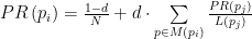 |
where
Equation 2 shows a matrix form of Equation 1. The matrix form is most likely the form used "out in the wild."
| Eq. 2 |  |
where
Note that many examples of PageRank are computed using a variant of Equations 1 and 2 that multiplies the PageRank value by the number of pages (N ·PageRank). Equation 3 illustrates Equation 2 modified with the substitution 
| Eq. 3 |  |
 |
|
 |
There has been quite a bit written about the nuances of this equation because of its importance in determining a web page's position in a list of search results. I am not concerned about those details here. I am focused here on the calculation of the PageRank for a specific set of pages.
My son was using Ian Roger's excellent site for learning about the details of PageRank. The question he had is on Example 10, which assigns a PageRank of 1 to an external page. Figure 1 shows the Example 10's web page configuration. Ian's PageRank results are shown in the boxes, which represent web pages. I want to show the details on obtaining Ian's results as an illustration of how to handle an external link from a page with a defined PageRank.

Figure 1: PageRank Example from Ian Roger's Website.
When Ian uses a link from an external site, he sets the PageRank value to 1. Here is his rationale.
We'll assume there's an external site that has lots of pages and links with the result that one of the pages has the average PR of 1.0.
Algebraically, this is easy to handle. Figure 2 shows my solution implemented in Mathcad.

Figure 2: Algebraic Solution for Example 10.
Figure 3 shows how I setup my iterative solution. To force page A to have a PageRank of 1, I needed to remove page A from the R vector and M matrix, but add it back in so that page A's contribution can be included. Again, it is a slight modification of Equation 3 so that I can force page A to have a PageRank of 1.

Figure 3: Setup for My Iterative Solution of Equation 2.

Figure 4: Iterative Solution of Equation 2.
I obtained the same results as Ian using two different approaches -- algebraic and iterative. This example was different than most in that a particular web page was forced to a particular PageRank. I hope that I answered my son's question.
I saw a bolide meteor while driving out to Montana last week. For those who are not familiar with bolide meteors, the Wikipedia has a nice description.
The word bolide comes from the Greek βολίς (bolis) [2] which can mean a missile or to flash. The IAU has no official definition of "bolide", and generally considers the term synonymous with "fireball". The term generally applies to fireballs reaching magnitude −14 or brighter.[12] Astronomers tend to use "bolide" to identify an exceptionally bright fireball, particularly one that explodes (sometimes called a detonating fireball). It may also be used to mean a fireball which creates audible sounds.
I have seen two bolide meteors in my life. I saw my first one while walking home from Catholic education one evening during 8th grade. It was very bright and lasted only a short period of time. About 30 seconds after it vanished, I heard a rumble. Next day, the local newspaper reported that a meteor had been spotted and fragments had been picked up on the ground.
Last week, I was driving late in the evening when I saw a bright white streak come across the sky that appeared to drop a yellow and then a green fragment. I have watched meteors my whole life and this was the first time that I saw colors. I did not know that others have seen colors until I saw this article. This was pretty cool!
I have an application where a potentiometer may be useful. In fact, it would be useful if the potentiometer had a logarithmic resistance characteristic, which is also called an audio taper for reasons that I will cover later. I have never used a potentiometer with a logarithmic characteristic before and I thought it would be worth documenting what I learned during this effort.
What is normally referred to as a logarithmic taper is really an exponential characteristic. A typical logarithmic taper potentiometer characteristic is shown in Figure 1 (Source).

Figure 1: Example of A Logarithmic/Audio Taper Potentiometer Resistance Characteristic
Each vendor will have a different "series" label for the logarithmic potentiometers, which often have names like "series A" or "series W." The series designation indicates a different set of resistance curves.
Not all vendors include a graph of the resistance characteristics of their logarithmic potentiometers. Many of the vendors include a specification that says something similar to the following quote (source):
The “W” taper attains 20% resistance value at 50% of clockwise rotation (left-hand).
This specification means that the potentiometer has
This type of specification gives you sufficient information to create an exponential curve fit, which I illustrate in Figure 2.

Figure 2: Illustration of the Fitting of an Exponential Function to the Specified Points.
The math associated with this curve fitting is shown in Figure 3.

Figure 3: Curve Fitting Math.
Equation 1 illustrates the basic form of the logarithmic potentiometer's resistance characteristic R(x), where x is the wiper position as a percentage of full scale.
| Eq. 1 |  |
where
The logarithmic taper is commonly called an audio taper because it is often used audio applications for loudness control. Understanding why involves knowing a little bit about human hearing. Figure 4 (Source) illustrates a human's perception of loudness relative to the Sound Pressure Level (SPL). Sound pressure level is proportional to an audio amplifier's output power. However, the ear is sensitive to the log of the sound pressure level. This is why the "logarithmic" taper is useful.
.")
Figure 4: Loudness Level Versus Sound Pressure Level (dB).
When people are adjusting the loudness of their audio gear, they prefer that the loudness increase by an amount proportional to amount of dial or slide movement. If a linear potentiometer is used to control output power (and therefore loudness), you will need to use larger and larger amounts of wiper movement to get the same loudness change. To get the same amount of loudness change for a the same amount of wiper movement, the potentiometer resistance needs to increase exponentially.
Figure 5 shows what how the loudness is perceived by a person as the potentiometer's wiper is moved. You can see that the perceived loudness increases approximately linearly for wiper positions above ~20%.

Figure 5: Potentiometer Resistance Model and Linearized Loudness Characteristic.
After all this research, I ended up not using the logarithmic potentiometer because it was not logarithmic. I ended up using another approach which I will discuss in a later post.
I used to watch the television show "MASH" years ago. They would refer to quick procedures for patient stabilization as "meatball surgery." I recently encountered some "meatball math" as part of my engineering job. I call it "meatball" because the "patient", a recalcitrant laser, had to be fixed quickly and rough approximations were totally acceptable. This application was a nice application of Mathcad and the implementation of the approximation in C will soon be going out in one our software loads.
We use AVR processors from Atmel to perform simple controller functions. I like these processors so much that I have an AVR development system at home (you never know when you might want to cookup some controller code). In one of our products, we need to estimate the threshold current for a laser at a given temperature. It turns out that Equation 1 [Keiser] does a fair job of modeling the temperature variation of the threshold current.
| Eq. 1 |  |
Equation 1 requires the computation of an exponential function. Unfortunately, a library version of the exponential function requires lots of memory space and my available AVR memory space is very small. However, it turns out that I do not need tremendous accuracy in this application – ±2% would be fine. I started to think in terms of a piecewise linear approximation. Let's take a look at what this approximation involves.
We begin with some simple algorithm requirements:
As always, I began my work by seeing if anyone else has already solved my problem. My first search turned up an article on a bifurcated linear approximation to the exponential function over the input range 0 to 1.
Figure 1 shows a plot of the bifurcated approximation. This equation meets my accuracy requirement, but it is not designed for my input range from 0 to 1.5. Let's use Mathcad to fix this.

Figure 1: Bifurcated Linear Approximation to the Exponential Function.
I needed to get this approximation out quickly, so I decided to augment the range setup of Equation 1 (0 to 0.5, and 0.5 to 1) with a third range (1.0 to 1.5).
Figure 2 shows the form of my linear function and my error function, which I will minimize. I am using the "minimax" optimality criterion for my approximation.

Figure 2: Linear Approximation Prototype and My Error Function.
We can use solver to find the optimal solution. Figure 3 shows my solution setup. Note that I randomly chose the starting values. I ended up trying various random starting values to come to my final choice of coefficients.

Figure 3: Trifurcated Mathcad Solver Setup.
Note how I am also enforcing a continuity requirement at the end points of my ranges. The bifurcated solution did not enforce this criterion and their error function was not smooth. Figure 4 shows the results of my Mathcad work.

Figure 4: Plot of My Trifurcated Linear Approximation to the Exponential Function.
The equation shown in Figure 4 solved my problem. This was a good example of a "quick and dirty" solution to a common engineering dilemma -- an accurate solution is too big or expensive and you need to find an approach that is good enough. That is exactly what was done here.
I am doing some interesting work with lasers this week. I thought it would be useful to provide some background on how we build and control lasers. We deploy a lot of lasers in outdoor applications, which means that special attention must be paid to the temperature characteristics of lasers. If you are a small business that is considering getting a laser cutter then you should probably do your research to understand better how laser cutters work, you could take a look at something like this best laser cutter for small business to show you what could be offered to you. Keep on reading though to find out more about lasers, the automotive supply chain and how they work. Like batteries, lasers have characteristics that vary with temperature, with some industrial lasers needing products like North Slope needed to mitigate the heat and stabilize equipment for optimal laser performance. These temperature variations would cause the laser's output power to drop if actions were not taken to compensate for the temperature variations. These variations also make a laser subject to thermal runaway, also just like a battery. This week's work will focus on temperature compensation. But first, let's discuss how our lasers operate and are assembled. Once we have established that base, we can move on to related topics.
Lasers emit light when they are driven by current above a level called the threshold current (symbolically IThreshold). The more current you drive into the laser above the threshold level, the more optical power that the laser emits. Figure 1 illustrates this characteristic.

Figure 1: Idealized Laser Output Power Versus Input Current Characteristic.
Let's summarize the key points of Figure 1:
We can model this characteristic using Equation 1.
| Eq. 1 |  |
This power versus drive current characteristic by itself does not cause any problems. However, IThreshold and SE both vary with temperature and this is the source of my woes. Figure 2 shows how the laser characteristics vary with temperature for a real device. Notice how the slope efficiency reduces with increasing temperature. That is the key problem, as I will discuss below.

Figure 2: Slope Efficiency Graph for an Actual Laser.
Digital communications using fiber optics is similar to many other forms of digital communications in that we encode binary information by sending light down the fiber at two different power levels. The high-level is called a "1" and the low-level is called a "0". Figure 3 illustrates what an idealized optical bit stream looks like.

Figure 3: Example of a Digital Bit Stream Using Optical Power Modulation.
Because SE decreases with temperature, maintaining constant "1" and "0" levels means increasing the drive current with increasing temperature. It turns out that this is a more difficult problem to solve than you might think. Figure 4 shows how we convert drive current into optical power. We try to control two parameters:

Figure 4: Conversion of Drive Current Into Optical Output Power.
Over the years, we have used various temperature compensation techniques. It turns out that controlling a laser's output power near room temperature is simple. However, particularly at high temperature, problems develop because the drive current becomes so high that the laser self-heats. This self-heating results in lower SE, which means more drive current. The laser is now in thermal runaway, which means our control circuitry will need to shut down the laser to prevent damage.
We have used feedback to control the laser's average output power 
We have used a mathematical model for the variation of SE with temperature and have used this model to predict the required increase in the difference between the "1" and "0" drive levels with temperature. This has proven to be a mediocre solution. The temperature characteristics of a laser vary by vendor and lot. We need something better -- we need a two feedback loops. One feedback loop to control average power and another to control the difference in levels between a "1" and "0". It turns out that a new "dual-loop" laser drivers are now becoming available. Future posts will discuss how these devices work.
Before I go too far into controlling a laser, let's talk about how commercial laser systems are constructed. Figure 5 illustrates how lasers are typically configured for use in communications applications. The laser is mounted so that the vast majority of the optical power generated goes into the fiber, with a tiny fixed percentage tapped off for measurement by a photodiode (called the monitor photodiode). In Figure 2, the light going to the left is focused into fiber by some type of lens, which is commonly a ball lens but can be other types.

Figure 5: Standard Laser Configuration for Communications Applications.
Figure 6 shows how lasers are packaged into transistor-outline (TO) cans, which is how we often see them.

Figure 6: Illustration of Laser TO-Can Packaging.
This post was intended to provide some background for the posts to follow. These posts will look at applying lasers in communications applications.
I was listening to a news program this weekend when I heard a journalist say that "4 million babies are born in the US every year." When I heard that statistic, I thought that I should be able to estimate that number using generally available information. Another Fermi problem!
But before we begin, I was inspired to write this post after speaking to two of my best friends. They have just had a baby and I got to meet her for the very first time a few days ago. She might only be a few months old, but already her parents have started playing educational songs and YouTube videos to keep her entertained! They are big believers in the notion that babies learn through music and I have to admit, some of the songs were pretty catchy so I can definitely see the appeal.
Now, baby news to one side, let's see if we can come up with a rough estimate of the number of babies born in the US every year. Here is my line of reasoning.
I was able to estimate that 4 million babies are born in the US each year using generally available information. This agrees nicely with the actual value of 4,055,000 (2010). Whenever I hear a statistic, I always like to think about it and see if it makes sense. Hearing that 4 million babies are born in the US each year now makes sense to me.

Figure 1: Terrence Tao with Paul Erdos.
While on my vacation to Ireland, I brought along a book called "Solving Mathematical Problems: A Personal Perspective" by Terence Tao. The book was written when Tao was a 15 year old mathematics prodigy competing in international mathematics competitions. Today at 36, he is one of the world's top mathematicians.
I have really enjoyed reading this book. I work with a lot of folks on developing their problem solving abilities. In the past, I have used the books by Polya (here is one and another) on problem solving heuristics. While these books are good, I really like the tone of "Solving Mathematical Problems." Tao does a very good job of describing the experimental aspects of problem solving.
Many folks new to problem solving will see a fully formed solution and do not understand that there may have been quite a bit of trial and error involved in coming up with that solution. Thus, the most common question I get from these newbies is "how do I know where to start"? Tao addresses this question by including with his solutions a discussion of alternative approaches and why he chose not to use them. I really appreciate this style of presentation -- all in the voice of a 15-year old. It is conversational and pleasant to read.
The book is focused on the kind of problems encountered in mathematics competitions:
It is a small book, but filled with mathematical gems. If you decide to check it out, I think you will find it worthwhile.
Quote of the Day
Being president is like running a cemetery -- you've got a lot of people under you and nobody's listening.
- Bill Clinton
I have taken a break from blogging to do some traveling. You may have already noticed from my Instagram account. I've decided to start using it again. To be honest, I probably would've stayed off it for a bit longer hadn't it been for my friend who is starting to get a lot of followers to their account. I think they said they have enlisted the help of an instagram manager to assist with their growth, and I have to say it's definitely seemed to work. So, you could say that it was part of my decision to start using it again. It'll also allow me to remember those places and bring back memories. I only have one issue... I have zero followers?! I know there are ways to get free followers on sites similar to socialfollow so I may give that as a shot! But above all, the highlight of my travels has been a bus trip around Ireland. It was great! We spent 8 days on a bus driving all over Ireland (see Figure 1). We also spent 4 days on driving around Ireland on our own. I must admit that driving on the left-hand side initially worried me, but after a day of careful, thoughtful driving it started to feel normal.

Figure 1: Our Bus Ride Around Ireland.
The Irish could not have been nicer, but things are not easy over there. Their economy is in a shambles and the cost of living there is high -- I read a news article that stated that Ireland has the fifth highest cost of living in the EU. They have many of the same economic complaints as the folks in the US:
In the case of the Irish, their sadness is particularly profound because many feel that their chief export today is their young people – just as during the Irish Famine. Thank goodness that Australia has work for some of them. However, losing your young people because of economic conditions is a terrible thing to say about an economy.
During our trip, the impact of the potato on Irish history could not be ignored. While I have no Irish ancestry (my wife has all the Irish blood), I do feel a kinship with the Irish in regards to the potato. I was raised in a small town that was surrounded by potato fields, my brother was a potato farmer, and I worked on a potato farm to earn money for college. When I was a boy, the potato farmers would proudly boast that no crop produced calories per acre like the potato. While apple growers may take exception, the potato does beat the grain crops handily. Consider the data in Table 1 for irrigated crops today. Yields at the time of the Irish Famine were substantially less.
| Crop | Millions of Kilocalories Per Acre |
| Soybeans | 2.1 |
| Wheat | 6.4 |
| Corn | 12.3 |
| Potatoes | 17.8 |
Potatoes were the calorie per acre leader back in 1846 as well.
Our bus stopped by the Irish National Famine Museum. It was very impressive place that provided us some insight to the living conditions at that time. During our tour, our guide discussed a number of Irish Famine facts:
Let's examine that calories per acre question a bit closer. How big an impact did the switch from potatoes to oats have on calorie production?.
Our Famine Museum tour guide mentioned that potatoes produce 2.5 times more calories per acre than oats. Let's try to understand where this number comes from because it is critical to understanding the Famine.
Given this information, the calorie comparison between potatoes and oats can be performed as shown in Figure 2.

Figure 2: Comparison of the Calories Per Acre Between Potatoes and Oats.
So I now understand the calorie difference between potatoes and oats. If we assume that the Irish tenant farmers were growing their personal food on the same acreage as before, the switch from potatoes to oats meant that the land could now only support 40% of the existing population. One solution to the problem would have been to stop exporting crops and use those crops to feed the Irish. The landlords did not do this. They simply chose to let the Irish starve.
Sadly, the Irish Famine was completely unnecessary. It turns out that there was plenty of food in Ireland to feed the people, but the landlords needed to export the food in order to keep their incomes up. The attitude of the government is summed up by the following quote (Reference).
The economists then concluded that since all the demand side measures had failed, nothing could be done. The only way to prevent future famines was to reduce demand, by "letting nature take its course". "‘I have always felt a certain horror of political economists,' said Benjamin Jowett, the celebrated Master of Balliol, ‘since I heard one of them say that he feared the famine of 1848 in Ireland would not kill more than a million people, and that would scarcely be enough to do much good.' The political economist in question was Nassau Senior, one of the Government's advisers on economic affairs." (Woodham-Smith 1991 pp 375-6). He need not have worried: 2.5 million people died out of a population of 8 million.
You might wonder how the British were able to export food with starving people all around. Here is another quote that describes that situation (Reference).
Ireland starved because its food, from 40 to 70 shiploads per day, was removed at gunpoint by 12,000 British constables reinforced by the British militia, battleships, excise vessels, Coast Guard and by 200,000 British soldiers (100,000 at any given moment)