
Quote of the Day
Acting was fun, but my grandfather would always tell me, "It's never too late to be an engineer." You were supposed to get a "job" and do acting on weekends or at school.
— Jon Hamm
Introduction
I was at dinner last night with some neighbors and the topic of hiring came up. My most important job is hiring the right engineering talent. When it comes to engineers, people frequently focus on their technical skills. While that is important, their ability to work with others is just as important. There are also some personality characteristics that I look for as well. The best engineers that I have worked with have these personality characteristics in common.
Personality Metrics
I am an engineer who writes a math and science-oriented blog, so I have to have some form of math even for personality characteristics. I evaluate the personality characteristics of an engineer using three personality metrics:
- Anality
- Pisstivity
- Prima Donnas Per Square Foot Factor
Anality
I frequently hear people say that they do not want to get wrapped up in the details of a problem. I always respond that my job is a celebration of detail. Many an engineering project has been destroyed because minor details were not attended to. I expect an engineer to be detail-oriented. The really good engineers know how to move from high-level to low-level thinking as the situation requires.
Pisstivity
Pisstivity is about owning problems. Anyone who has used contract labor understands this problem. Contractors can be very skilled, but they usually are not personally invested in the problems they are working on. Some employees have the same attitude. I look for engineers who have a history of looking for problems, grabbing them, educating themselves about the problem, and owning it all the way to the solution.
Many times I have had to ask someone to take on a problem in an area for which they have no skill. That is just the way life is sometimes. I have always been impressed with those staff members who, instead of griping, treat the situation as an opportunity to expand their skills and develop a new area of expertise. Managers cherish these employees.
Prima Donnas Per Square Foot Factor
This is really my "do they work well with others" index. Nothing disrupts a finely tuned engineering group more than a prima donna. Sometimes you need them but they need to be spread thinly – very thinly. The best engineers have egos, but they have been humbled enough that they know that nature is complicated and they just might be wrong. They also find ways to make all the people around them better, while the prima donna is all about him.
Conclusion
An engineering manager's most important task is hiring. The hiring of the right engineer can be a company-changing event. I have numerous stories of an engineer being hired by a company who literally changed the direction of the entire business. I will relate one story here.
When I was at HP in the old days, I remember a manufacturing engineer who thought that HP should be making low-end laser printers. His managers told him to go away. He then went off and bought a Canon copier mechanism and, on his own time and with his own money, built the first low-end HP laser printer. Grudgingly, management told him he might have something there and they turned it into a product. Today, HP is the world's largest manufacturer of printers. It all started with a young manufacturing engineer who would not give up. How is that for pisstivity!
")
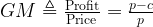

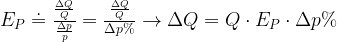
 is the percentage change in yearly shipment quantities.
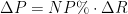
 is the percentage change in average selling price.
 ).
).


 is the wavelength range between the points at the SMSR level. Figure 1 illustrates how the measurement is made.

 )
) )
)
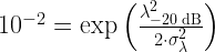

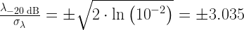
 is one of the two wavelengths where the spectral amplitude is down -20 dB from the peak. We define the
 , simply divide the
")


 is roughly the diameter of the umbra spot on the Earth. This completes my derivation.
 about the signal peak (
 total), the bit time will contain 95% of the normal pulse's energy.


 about the signal peak (


 a bit.
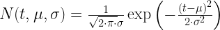
 is the standard deviation and
  is the mean of the normal curve. The Wikipedia has a nice graph of the normal curve, which I include in Figure 2.
")

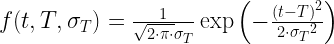
 is the wavelength,
  is the center wavelength of the pulse,
  is the standard deviation of the pulse width in time, and
  is the standard deviation of the pulse width in wavelength. For this discussion, we are going to ignore attenuation losses and focus on the effect of dispersion. It turns out that the losses due to attenuation are easy to add, but they add more bulk to this discussion that is already too long.
 .
.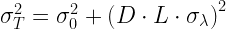
 is the time-domain variance of the total waveform,
  is time-domain variance of the initial pulse (t=0), L is the distance of pulse travel, and
  is the standard deviation of the laser pulse.

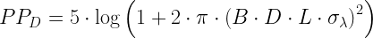
 . This reduction in pulse amplitude means a reduction in power that can be modeled using Equation 7.
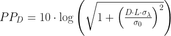
 , we can derive the
 , we can solve Eq. 8 for

 ). Figure 1 illustrates how the pulse distorts as it moves down the fiber.


 is the speed of light in glass
 is the index of refraction


 is the density of water (1 gm/cm3
 is the
