Math Encounters Blog

Compensating GPS Clocks for the Effects of Relativity

Posted on 1-June-2015 by mathscinotes

What you are will show in what you do.

— Edison

Introduction

Figure 1: Block 3 GPS Satellite. These satellites
have changed many aspects of our lives,
everything from land surveying to car driving
and flying airplanes (Source).

I occasionally read articles on Stumbleupon and I came across an interesting article called "8 shocking things we learned from Stephen Hawking's book" – the book they are referring to is called The Grand Design. I personally would not call the statements in the article shocking, but that is just my opinion.

However, there were two factoids that I thought were interesting and I would write posts about. This post will be about the following statement on relativity and the GPS system (Figure 1).

If general relativity were not taken into account in GPS satellite navigation systems, errors in global positions would accumulate at a rate of about ten kilometers each day.

I read a paper quite a while ago on the topic and I recalled that there is ~14 kilometer per day error due to general relativity effects, and ~2 km per day of error in the opposite direction for special relativity, for a total error of ~12 km per day. So I thought I would work through the math behind these effects and present the results here.

Background

General Information

If you are looking for more background on GPS errors, the Wikipedia as a very good article on the magnitude of the relativistic errors in GPS on this page. My approach here will be to work through the equations and material shown in Figure 2 of this post, which presents a slightly different viewpoint on the same material. Figure 2 contains an equation for computing the frequency shift due to general relativity that I have not worked with before and I will derive it as part of my work here.

Infographic on GPS Satellites

Figure 2 shows an infographic from Hugo Fruehauf, one of the key GPS developers. In this graphic, he mentions a daily timing correction of 38.6 µsec for relativistic effects. When I heard this timing correction, I quickly multiplied it by the speed of light to get the equivalent distance error (Equation 1).

Eq. 1

$\displaystyle {{d}_{r}}=c\cdot \Delta {{t}_{r}}=3.8\cdot {{10}^{8}}{\frac{\text{m}}{\text{s}}}\cdot 38.6\mu\text{sec = 11}\text{.6 km}$

where

Δt_r is the daily GPS timing correction required for the combined effects of general and special relativity.
d_r is the distance error due to the combined relativistic effects.
c is the speed of light in a vacuum.

Figure 1: Infographic from a Presentation I Saw on GPS.

Figure 2: Infographic from a Presentation I Saw on GPS.

General Relativity Effect on GPS Clock Frequency

Because a clock on earth is subject to a stronger gravitational field than the satellite, the clock on the satellite will appear outrun the same clock on the earth. We can use Equation 2 to determine the impact of gravitational time dilation on the clock frequency at different distances from the center of a gravitational field.

Eq. 2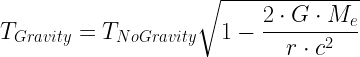

$\displaystyle {{T}_{{Gravity}}}={{T}_{{NoGravity}}}\sqrt{{1-\frac{{2 \cdot G \cdot M_e}}{{r \cdot {{c}^{2}}}}}}$

where

T_NoGravity is the clock's period infinitely far from any gravitational field.
T_Gravity is the clock's period at distance r from the center of the gravitational field.
c is the speed of light in a vacuum.
M_e is the mass of the Earth.
G is the universal gravitational constant.

While the GPS clock is in orbit, we will need to know its period as measured from the Earth. However, the the influence of gravity will cause the apparent clock period to change when it moves from the Earth into orbit. We can compute the clock period shift due to the effects of general relativity by using Equation 2 and working with the differences in the clock periods at the radii of the Earth's surface and the satellite's orbit.

Special Relativity Effect on GPS Clock Frequency

Because a clock on the satellite is moving relative to the same clock on the earth, the clock on the satellite appears to run slower than the same clock on earth. The clock period on the orbiting satellite (T_SatSpec), is longer than the clock period (T_EarthSpec) for the same clock at rest on Earth (Equation 3).

Eq. 3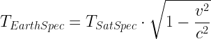

$\displaystyle {{T}_{{EarthSpec}}}={{T}_{{SatSpec}}}\cdot \sqrt{{1-\frac{{{{v}^{2}}}}{{{{c}^{2}}}}}}$

where

v is the speed of the moving observer.
T_EarthSpec is the clock period measured for a GPS clock on Earth.
T_SatSpec is the clock period for a GPS clock mounted on a "fast" satellite and measured by an observer on Earth.

The clock period correction required for special relativity is in the opposite direction as the correction for general relativity.

Analysis

Percentage Frequency Change Due to General Relativity

Figure 3 shows my derivation of a formula for the percentage frequency shift due to the effects of general relativity. My results agree with those shown in Figure 2.

Figure 3: Derivation of General Relativity Percentage Frequency Change.

Percentage Frequency Change Due to Special Relativity

Figure 4 shows my derivation of the formulas and results for the percentage clock frequency change caused by the effects of special relativity. My results agree with those shown in Figure 2.

Figure 4: Derivation of Percentage Frequency Change Due to Special Relativity.

Combined Frequency Change

Figure 5 shows the combined frequency error effects of general and special relativity and how they result in a distance error of about ~12 km per day.

Figure M: Combined Relativistic Effect on Clock Rate and Effective Distance Error.

Figure 5: Combined Relativistic Effect on Clock Rate and Effective Distance Error.

Conclusion

I was able to show that the combined effects of general and special relativity produce ~12 km worth of distance error per day into the GPS system that must be accounted for. This agrees with the quote from the Stumbleupon article.

For a very good history of the GPS program, see this document.

Save

Posted in Navigation | 5 Comments

Range Table Construction Using Pejsa's Formulas

Posted on 28-May-2015 by mathscinotes

I've missed more than 9000 shots in my career. I've lost almost 300 games. 26 times, I've been trusted to take the game winning shot and missed. I've failed over and over and over again in my life. And that is why I succeed.

— Michael Jordan

Introduction

Figure 1: Godzilla Returning to the Sea (Source).

This is my final, planned post on Pejsa's ballistic model. I feel a little like Godzilla (Figure 1) marching back into the sea at the end of one of his many movies – it is time to move on to other subjects.

In the main body of this post, I work through a detailed example from "Modern Practical Ballistics" on how to apply Pejsa's formulas to determine a range table for a projectile moving through a wide range of velocities. In Appendix A, I work through a second example from the text as additional validation of my implementation. In Appendix B, I show how to use an Ordinary Differential Equation (ODE) solver to generate a range table for comparison with Pejsa's algebraic approximations.

Background

While I have mentioned some of the following concepts before, a little review will not hurt.

Velocity Zones

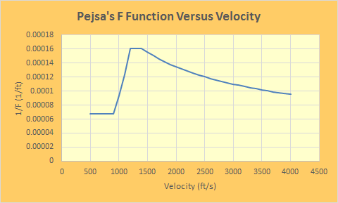
One projectile modeling complication is that the functional dependence of drag on a projectile varies with the velocity of the projectile. Pejsa modeled drag using formulas of the form ${{F}_{{Drag}}}\propto {{v}^{{2-n}}}$ with different values of n defined in four velocity zones . The velocity zones and the associated values of n are defined as:

zone 1: 1400 ft/s to 4000 ft/s
This is the supersonic velocity zone and n= 1/2 in this region.
zone 2: 1200 ft/s to 1400 ft/s
This is part of the low supersonic region and n=0 in this region.
zone 3: 900 ft/s to 1200 ft/s
This is part of the transonic region and n = -3 in this region.
zone 4: 0 ft/s to 900 ft/s
This is the subsonic region and n=0 in this region.

Figure 1 illustrates the F curve used by Pejsa, which describes the deceleration of the reference projectile.

Figure 2 Pejsa's Velocity Zones.

Drop Rate

Before I get too far, I need to define a term that Pejsa called the "drop rate".

Drop Rate (D_R): The drop rate is the number of vertical inches a projectile drops per yard of horizontal travel.

Pejsa computes the drop rate at the end of each velocity zone. The drop rates accumulate as the projectile passes through each velocity zone. We can use Equation 1 to compute the drop rate of the projectile at the end of a velocity zone. This rate will persist in the projectile from the end of the velocity zone to the final range.

Eq. 1

$\displaystyle \frac{{dD}}{{dR}}=\frac{{2\cdot D}}{R}\cdot \left( {\frac{{1+0.78\cdot n\cdot {{{\left( {\frac{R}{F_m}} \right)}}^{2}}}}{{1-\frac{R}{F_m}}}} \right)$

where

F_m is the mean coefficient of retardation (feet).
D is the drop at range R for a projectile fired horizontally (inches).
n is the exponent correction associated with the velocity zone the bullet just passed through (unitless).
R is range the projectile has traveled through the current zone (yards).

Equation 1 is derived in Appendix C.

Pejsa's Solution Approach

Pejsa's approach can be summarized as follows:

Treat each velocity zone as a separate problem.
This means that we develop separate solutions for velocity zones 1, 2, 3, and 4 as if the other zones do not exist. This would be equivalent to firing a projectile four times with velocities
- V₀, the muzzle velocity.
- 1400 feet per second (fps), the velocity at the high–end of zone 2.
- 1200 fps, the velocity at the high–end of zone 3.
- 900 fps, the velocity at the high–end of zone 4.
While this part of the solution does not assume that height change is affected by the projectile passing through previous regions, in fact, there is a strong interaction. This interaction can be modeled separately as shown below. My discussion will assume that the projectile traverses all four velocity zones – it might not. If the projectile only traverses some of the zones, simply evaluate Pejsa's equations for the zones it does pass through.
Calculate the drop rate at the end of each zone.
The drop rate from the previous zone will carry forward into the next zone. We can compute its contribution to the height change by computing the product of the drop rate from the previous zone times the distance traveled.
Sum up all the contributions from gravity and drag in the current zone plus with the drop rate contributions of previous zones to get a total drop rate.
This gives us the rate of change of height relative to the line of sight with respect to distance. We can integrate this rate of height change function with distance to get the total change in projectile height.

Analysis

Example Source

Pejsa includes a large table of ballistic solutions in the back of his book for various projectiles. I randomly chose an example with a muzzle velocity V₀=2400 fps and a ballistic coefficient BC=0.4 to test my implementation of his equations.

Solution Setup

Figure 3 shows how I determined the ranges at which the projectile crosses from velocity zone into another. Calculations begin with the F function, which represents the deceleration of the reference projectile (i.e. a 1-inch diameter, 1 lb, G7 shape) at various velocities.

Figure 3: Critical Range Determination.

Drop Formula For Multiple Velocity Ranges

Now that I have computed the distances at which the projectile transitions from one velocity zone to another, I can compute the various drops that occur as a function of the ranges within each zone. Figure 4 summarizes these calculations. Observe that I compute the drop rate (y-direction) accrued by the end of velocity zones 1, 2, and 3. I sum all the drop contributions to the projectile in the function D_R.

Figure M: Implementation of Drop and drop rate Equations.

Figure 4: Implementation of Drop and drop rate Equations.

Generating a Range Table

Given the zone transition distances, the projectile drops due to gravity and drag, and the drop rates at the end of each zone, I can now compute the height of the projectile relative to the line of sight using the equation 2 from this post for a projectile's height (H) above the line of sight (Figure 5).

Figure M: Generate the Results Table and Compare Results.

Figure 5: Generate the Results Table and Compare Results.

My results show excellent agreement with Pejsa's results.

Conclusion

This concludes my planned review of Pejsa's "Modern Practical Ballistics". I have presented detailed derivations of his key results and provided examples of their application using Mathcad. Hopefully, the material presented here will be useful to those battling through Pejsa's book – it was one of the most frustrating reads I have encountered. I believe that I mastered the material, but that was in spite of the book's presentation.

Appendix A: Textbook Example

I have tried my routine on multiple examples from Pejsa's book. On page 94, Pejsa works an example and presents the results in Figure 13 of his text. I have used my implementation of his equations to duplicate his results in this example file (Figure 6). This file is a PDF of the same Mathcad routine used to generate the results in the main body of this post.

Figure 6: My Results and Comparsion with Chapter Example.

Figure 6: My Results and Comparison with Chapter Example.

Appendix B: Range Table Creation With ODE Solver

Pejsa's algebraic ballistic solutions are approximate solutions to the differential equations that describe the projectile's motion. I inserted Pejsa's differential equations into Mathcad, generated numerical solutions for a number of examples, and compared the results with the output from Pejsa's software. As you would expect, the agreement is excellent (Figure 7).

Figure M: Comparision Between DE Solver and Pejsa's Equations.

Figure 7: Comparison Between DE Solver and Pejsa's Equations.

I have attached a PDF of my worksheet Blog_ODE.

Appendix C: Derivation of the Drop Rate Equation

Figure 8 shows my derivation of the drop rate equation (Equation 1).

Figure M: Derivation of Drop Rate Equation.

Figure 8: Derivation of Drop Rate Equation.

Posted in Ballistics | 7 Comments

Optical SFP Power Estimation Using Curve Fitting

Posted on 26-May-2015 by mathscinotes

A leader is a man who has the ability to get other people to do what they don’t want to do and like it.

— Truman

Figure 1: Curve Fit SFP Power Data.

I was asked today how to use Excel to estimate the power usage of two optical components at case temperatures for which we had no data. I initially solved the problem in Mathcad by fitting an equation of the form $c_0 \cdot e^{c_1 \cdot T_{Case}}+e_2$ to the data and computing the corresponding power.

Since most of the engineers where I work do not use Mathcad, I was asked if I could demonstrate how to get the same answer using Excel. On the assumption that some of you may have similar problems, I have included my SFP_Power spreadsheet here that solves the problem using Solver, an Excel add-in. No macros were required to solve this problem.

Posted in Excel, General Mathematics | Comments Off

Pejsa Formula for Midpoint as a Function of Zero Range

Posted on 21-May-2015 by mathscinotes

You can't work a Biegert too hard.

— Statement by a football coach to my son, who thought he was working too hard during practice. The same football coach had coached my brothers. You do not want to hear a football coach make this statement.

Introduction

Figure 1: Lots of Algebra in this Post (Source).

This post will cover Pejsa's formula for the trajectory midpoint as a function of the rifle's zero range. Shooters often have a preferred zero range, like 100 yards or 200 yards. This formula allows the shooter to determine his midpoint range directly from the zero range. The midpoint range can then be used to determine the maximum bullet height above the line of sight, which can be used to determine the maximum bullet placement error.

Of all Pejsa's formulas, this one is the most algebraically challenging to derive, but the process was worthwhile to go through. For example, it was the first time that I had an actual application for the Cardano cubic equation solution.

Equation 1 shows Pejsa's midpoint formula as a function of the rifle's zero range.

Eq. 1

$\displaystyle M=F\cdot \left[ {1+C{{M}^{{\frac{1}{3}}}}\cdot \left( {{{{\left( {CZ-1} \right)}}^{{\frac{1}{3}}}}-{{{\left( {CZ+1} \right)}}^{{\frac{1}{3}}}}} \right)} \right]$

where

M is midpoint range (yards).
$CM=\frac{{Z\cdot F}}{{\left( {Dz+SH} \right)}}\cdot {{\left( {\frac{G}{{{{V}_{0}}}}} \right)}^{2}}$ is a temporary variable used to make writing Equation 1 simpler.
$CZ=\sqrt{{\frac{8}{{27}}\cdot CM+1}}$ is a temporary variable used to make writing Equation 1 simpler.
Z is the zero range (yards).
Dz is the projectile drop at the zero range when fired horizontally (inches).
SH is the height of the scope above the bore of the rifle (inches).
V₀ is the initial velocity (ft/s).
G is a constant (41.68).

Background

All the required background was supplied as part of this three-part series.

Analysis

Equation Setup

Figure 2 shows how we can use Pejsa's drop formula for a horizontal projectile to generate a cubic polynomial with one real solution.

Figure 2: Derivation of a Cubic Equation Used to Compute the Trajectory Midpoint Given the Zero Range.

Solution

In Figure 3, I solve the Cardano cubic equation for the real root. This is where the serious algebra occurs.

Figure 3: Solution to the Cardano Cubic.

Example

Here is an example of how I would use Equation 1 in a real-world application. In this case, given a zero range, I can compute the midpoint of the trajectory. Given the midpoint, I can compute the maximum height of the bullet along its trajectory.

Figure 4: Working an Example From the Back of Pejsa's Book.

Conclusion

With this post, I have now reviewed all the major formulas in Pejsa's work. The last exercise will be computing the range table for a projectile moving from supersonic to subsonic speed. I view this calculation as more of a bookkeeping challenge than anything else, but it is a bit confusing.

Posted in Ballistics | 1 Comment

Pejsa Trajectory Midpoint Formula Given a Maximum Projectile Height

Posted on 20-May-2015 by mathscinotes

The most amazing achievement of the computer software industry is its continuing cancellation of the steady and staggering gains made by the computer hardware industry.

— Henry Petroski

Introduction

Figure 1: Critical Trajectory Points (Source:Me).

Pejsa defines the trajectory midpoint as the range at which the projectile height reaches its maximum (Figure 1). Pejsa's midpoint formula (Equation 1) allows you to compute the midpoint given a specific maximum height (H_m).

Eq. 1

$\displaystyle M=\frac{1}{{\frac{G}{{{{V}_{0}}\cdot \sqrt{{{{H}_{m}}+SH}}}}+\frac{2}{F}}}$

where

V₀ is the projectile's initial velocity (ft/s),
H_m is the maximum projectile height above the line of sight (in),
SH is the height of the scope above the projectile's trajectory (in),
G is a constant (41.68),
F is what Pejsa calls the coefficient of retardation (ft).

The derivation is straightforward and I will not provide much additional commentary beyond the mathematics itself.

Background

All the required background was supplied as part of this three-part series.

It is worth commenting that this is the only derivation that I recall where Pejsa uses a horizontal line of sight. He is able to use a horizontal line of sight because he makes the observation that his horizontal drop formula actually works for a projectile going forward (drag inhibiting its forward motion) and backwards (drag enhancing its forward motion). It is an interesting aspect of the symmetry of the formula.

This means that the derivation assumes that the projectile is moving BACKWARDs from the midpoint and is dropping down to the muzzle under the force of gravity with drag accelerating it.

Analysis

Derivation

Figure 2 shows the derivation of the midpoint formula. Observe that the derivation makes an approximation based on a truncating a Taylor series expansion.

Figure 2: Derivation of Formula for the Trajectory Midpoint.

Example

Figure 3 shows a worked example from the tables in the back of Pejsa's book. The agreement was excellent.

Figure 3: Example Taken from Pejsa's Tables in the Back of His Book.

Conclusion

In this post, I derived and provided an example of Pejsa's midpoint formula. I have two more posts left in my Pejsa review odyssey:

Derive the maximum projectile height for a rifle zeroed at a range of Z.
Provide an example of the projectile height relative to the line of sight for a projectile moving from supersonic to subsonic speeds.

Posted in Ballistics | 2 Comments

Pejsa Bullet Height Versus Distance Formula For a Zeroed Rifle

Posted on 19-May-2015 by mathscinotes

I'm desperately trying to figure out why kamikaze pilots wore helmets.

- I heard a historian ask this question on the History Channel. I cannot think of a good reason for them to wear a helmet, either.

Introduction

Figure 1: Trajectory of Bullet Relative to the
Rifle's Line of Sight (Source: Me, done for the
Wikipedia). Note how the rifle is canted slightly
up for a flat line of sight.

In this post, I will review Pejsa's development of a formula for the height of a bullet relative to the shooter's line of sight, assuming that the rifle is adjusted to have zero height at a known range (referred to as the rifle's "zeroed" range). Figure 1 illustrates the trajectory of a bullet fired from a rifle zeroed at a given range. If you're not familiar with how to zero a rifle scope at 100 yards, visit a website like riflescopescenter.com to learn more.

This formula is a straightforward extension of Pejsa's drop formula for a bullet fired horizontally (post). I will provide a derivation of the formula and show that I can duplicate some of Pejsa's published examples.

Background

Pejsa's Objective

Pejsa showed that you could determine the trajectory given the following information:

bullet's ballistic coefficient
bullet's initial velocity
sighting approach (two methods covered)
- zero the rifle at a specific range, or
- specify maximum excursion of the bullet above the line of sight

For this post, I will assume a known zero range. Pejsa goes into some detail on how to use the zero range to determine the maximum bullet height and vice versa. This is useful to shooters who want to know their placement error for a given zero range.

Drop Formula For Horizontally-Fired Projectile

Our goal in this post is to derive Equation 1, which is Pejsa's approximate solution to his projectile drop equation that we developed in Part 1.

Eq. 1

$\displaystyle \sqrt{D}=\frac{{\frac{G}{{{{v}_{0}}}}}}{{\frac{1}{R}-\frac{1}{{{{F}_{m}}\left(R\right)}}}}$

where

D is the projectile drop [inches].
v₀ is the initial projectile velocity [ft/sec].
R is the projectile horizontal travel distance [yards].
G is a constant with value 41.697 [ft[sup]0.5[/sup]/sec].
F_m (R)= F₀-3 n R/4 (I call this the "standard form").

Analysis

Range Equation

Pejsa uses Equation 2 to model the bullet's height above the LOS, which is based on the bullet drop formula for a horizontally-fired projectile.

Eq. 2

$\displaystyle H=-\left( {S+D} \right)+R\cdot \frac{{S+{{D}_{Z}}}}{Z}$

where

H is the bullet's height above the line of sight.
R is range at which we want the bullet height relative to the line of sight.
Z is range at which the rifle is zeroed.
D=D(R) is the bullet drop at range R given by Equation 1.
D_Z is the drop of a horizontally fired bullet at the Z range.
S is the height of the scope above the barrel.

Pejsa is able to use Equation 1 because, for calculation purposes, he assumes a slightly different shooting scenario than is illustrated in Figure 1. Figure 2 shows that model for the flight path assumed in deriving Equation 2. Observe that it is a rotation of the situation shown in Figure 1. Pejsa assumes that the rotation is so small that an errors introduced are minimal, which is a good assumption for the flat trajectory situation

Figure M: Model for Pejsa's Range Table Formula.

Figure 2: Model for Pejsa's Range Table Formula.

A bit of geometry is required to derive the formula, which I show in Figure 3.

Figure 3: Deriving the Height Versus Distance Formula.

Mathcad Model

Figure 4 shows how I computed a range table using Equations 1 and 2.

Figure 4: Calculation of Range Table Example.

Results

Table 1 shows my results versus the output from Pejsa's software for a projectile with

BC=0.4
V0=2900 feet/sec
n=1/2 (i.e. data tabulated at ranges where velocity is greater than 1400 feet/sec)

The agreement is nearly perfect to the first decimal place, which I consider good considering that we are interpolating the F function differently.

**Table 1: Bullet Height Computed Using Pejsa Software and My Mathcad Model.**
Range (yd)	Pejsa Software (in)	Mathcad Version (in)
0	-1.5	-1.5
50	0.3	0.3
100	1.0	1.0
150	0.5	0.5
200	-1.4	-1.4
250	-4.8	-4.8
300	-9.8	-9.8
350	-16.5	-16.5
400	-25.2	-25.2
450	-36.1	-36.0
500	-49.3	-49.2

Conclusion

I am nearing the end of my review of Pejsa's "Modern Practical Ballistics". The last items to cover will be

deriving an algebraic expression for the trajectory mid-range (i.e point of maximum bullet height),
deriving an algebraic expression for the zero point as a function of the maximum bullet height,
One worked example showing how to deal with a projectile moving from supersonic to subsonic.

Posted in Ballistics | 5 Comments

Untold ER Story About Tainted Well Water

Posted on 14-May-2015 by mathscinotes

When you drink from the well, remember those who dug the well.

— Chinese proverb

Figure 1: Spreading Fertilizers Can Contaminate
Ground Water with Nitrates (Source).

I sometimes wonder if you can learn anything from television, but I recently saw an article in our local paper about a medical condition threatening a local town that I had first learned about on "Untold Stories of the ER" (USER).

The USER segment was called "Blue Baby Syndrome" and it was about a 1 year old baby that developed a condition called methemoglobinemia, which can occur when drinking well water contaminated with nitrates – often by a local farmer's fertilizer. I have always wondered if fertilizers could contaminate well water and it turns out they can.

The Wikipedia defines methemoglobinemia as follows.

Methemoglobinemia is a disorder characterized by the presence of a higher than normal level of methemoglobin .... This leads to an overall reduced ability of the red blood cell to release oxygen to tissues, with the associated oxygen–hemoglobin dissociation curve therefore shifted to the left. When methemoglobin concentration is elevated in red blood cells, tissue hypoxia can occur.

Here is a short excerpt from the show.

The doctors did some nice detective work discovering that the baby was being exposed to nitrates in the water it was receiving in its formula.

While I saw the television show a few years ago, the article I saw was in one of our local newspapers (link) on the exact same problem being faced by an small Minnesota town.

Post Script

A frequent reader told me that when his mother was raising kids on the family farm in southern Minnesota many decades ago, local doctors warned the locals not to give babies well water for this exact reason. Apparently, it was well known a long time ago that well water contaminated with fertilizers was very bad for babies.

Posted in Health | Comments Off

Radioactive Paper?

Posted on 13-May-2015 by mathscinotes

I don't believe there is intelligent life on other planets. I believe they are just like us.

— A spacecraft designer whose name I don't recall.

Introduction

Figure 1: Glassware that Glows from Uranium Radioactivity (Source).

I probably shouldn't be surprised when I read that common materials are slightly radioactive. I am seeing an article on this topic every few weeks. For example, a few weeks ago I read an article about a type of glassware that contains a small amount of uranium and is slightly radioactive. It also fluoresces when exposed to UV light.

Figure 2: MINER Neutron Imager. Using omnidirectional imaging, MINER was able to localize a radiation source in a building in Chicago (Source).

I speculate that one of the reasons that I am seeing more articles on this topic is because governments around the world are putting radiation monitors at their ports of entry (example) and these detectors are occasionally flagging shipments of kitty litter and Brazil nuts.

These radiation detectors can be quite complex. Figure 2 shows an example of a neutron detector used for detecting, classifying, and localizing fissile material.

I just read an article article that glossy paper is also slightly radioactive, a fact that I found surprising. As I read about glossy paper, it turns out that glossy paper often contains kaolin, a type of clay. So it is radioactive for the same reason that kitty litter is radioactive, which also contains clay.

Figure 3: Radiation Spectrum of a Playboy Magazine (Source).

Most of the print magazines I read today are filled with glossy paper. Much of that paper comes from the forests near my cabin in northern Minnesota, where there are large paper plants that specialize in making glossy paper.

Figure 3 shows a radiation spectrum for a 400 gram Playboy magazine – clearly the researchers are men with a sense of humor. You can see the various radiation count spikes in their data at the energy levels for:

²³⁴Th (93 keV)
²¹²Pb (238 keV)
²⁰⁸Tl (583 keV)
²¹⁴Bi (609 keV)
²²⁸Ac (911 keV)

My long-term goal is to understand the radiation exposure that people on Earth are exposed to everyday and how those numbers differ from a place like Mars. As part of this effort, I will duplicate the author's calculations for the radiation exposure that a human would experience holding a magazine 1 foot away from their body for an hour.

The article presents the following radiation activity information for the magazine's paper.

0.15 to 0.35 pCi/gm (pico-Curies per gram of magazine ) of uranium isotopes.
I should discuss units a bit. The modern unit of radioactive decay is the Becquerel (Bq). One Bq equals one decay event per second. In the old days, radioactive decay was measured relative to radium and the unit of measure was called the Curie (Ci). One Ci equals 3.7E10 decays per second. This unit proved far too large for common usage and most folks ended up using pico-Curies (pCi).
0.3 to 0.6 pCi/gm of thorium isotopes.

These activity levels are not difficult to estimate. For example, I estimate the activity level from paper due to thorium in Figure 4. All the data came from a couple of web searches.

Figure X: Glossy Paper Activity Level Due to Thorium.

Figure4: Glossy Paper Activity Level Due to Thorium.

Let's assume that all the radiation activity is due to the paper's clay component, which contains uranium and thorium. If we assume that the magazine's mass is 400 grams, we can estimate the overall radiation level as shown in Figure 5.

Figure X: Activity Level from a Glossy Magazine.

Figure 5: Activity Level from a Glossy Magazine.

I then took this data and put it into the web-based radiation exposure calculator shown in Figure 6. The background behind what the calculator does is given here.


Figure 6(a) Thorium Series Calculations.	Figure 6(b) Uranium Series Calculations.

Figure 7 shows my calculation of a total radiation exposure rate of 0.0015 µREM/hour. This agrees with the results presented in the article.

Figure X: Final Result of 0.00015 µREM/hour.

Figure 7: Final Result of 0.0015 µREM/hour.

Posted in General Science | 3 Comments

Good Analogy for A VPN

Posted on 12-May-2015 by mathscinotes

Nothing in this world can take the place of persistence. Talent will not; nothing is more common than unsuccessful men with talent. Genius will not; unrewarded genius is almost a proverb. Education will not: the world is full of educated derelicts. Persistence and determination alone are omnipotent. The slogan 'Press On' has solved and always will solve the problems of the human race.

- Calvin Coolidge

Figure 1: World War 2 Navajo Code Talkers (Wikipedia).

My oldest son is an IT engineer and I find his work very interesting. So that we have more things to talk about, I am trying to become more knowledgeable about IT matters. This means I try to read various blogs about IT topics.

Today, I was reading the Kaspersky blog, and they had a great analogy for a Virtual Private Network (VPN). They said that the WW2 use of Navajo code talkers is analogous to a modern VPN.

For those who aren't quite sure what a VPN actually does, it's most commonly used to hide a computer user's IP address or location from the internet provider or server. If you want to learn more about how VPNs function, it might be worth reading this betternet review. In any case, VPNs provide the convenience of changing the location, which can be useful to access information or data that normally wouldn't be available to you. In practice, people use VPNs to access content on streaming services or websites that aren't available in their countries due to targeted geofencing. It is particularly visible with torrents (one of the main forms of P2P file sharing), in the manner in which they have been curtailed in recent years. A secure VPN connection, in this case, can protect users seeking large disk content, gaming isos from unwanted snooping. Another application of VPNs is in enhancing gameplay in video games. You may be looking at how to change location in pokemon Go, for example, in order to catch new pokemon.

Whilst VPN's are used for modern activities, they haven't changed much since coding was invented. Just like a modern VPN, the Navajo VPN had:

communication that occurred over an open network.
had a well-defined protocol.
encrypted communication so that only those with the "key" can understand what is being said.

I really like this analogy. While the Navajo code talkers may be the most famous example of using a spoken language as an encoding system, there actually are many other examples.

In the event a non-code talker Navajo was captured by the Japanese and forced to translate the code talker messages, the code talkers added an additional level of encryption to the messages in the form of code words. This practice is known as multiple encryption. For example, a tank would be called a turtle. A non-code talker Navajo actually was captured, and the poor man was tortured further because he could not translate the messages.

Posted in Networking | 2 Comments

Pejsa's Projectile Drop Versus Distance Formula (Part 3 of 3)

Posted on 11-May-2015 by mathscinotes

The Roman emperor creates catastrophes for Rome and calls them successes.

— Celtic warrior's words about the Romans. Sounds like today's politicians.

Introduction

Figure 1: Great Photo of Bicycle Acrobatics (Source).

In this post (part 3), I will work an example from Pejsa's "Modern Practical Ballistics 2^nd ed." and show that the exact and approximate solutions to the drop differential equation give nearly the same answers.

While the results presented here are accurate for a projectile fired horizontally, projectiles are normally aimed using sights that are "zeroed" for specific ranges (Figure 2). Most drop versus range tables assume the rifle is zeroed at a specific range.

Figure 2: Effecting of Zeroing on the Projectile's Trajectory

Figure 2: Effecting of Zeroing on a Projectile's Trajectory (Me, for the Wikipedia).

Zeroing involves adjusting your sight so that the projectile' s trajectory is given a slight upward tilt, which means the rifle's aim can be adjusted so that the bullet will strike where it is aimed for a specific range value.

Pejsa presents a modification of his horizontal drop formula that accounts for the effect of zeroing, but I will not be covering that material here – the extension is straightforward but a bit tedious. It may be material for a later post.

Background

Reference Projectiles

Pejsa's ballistic formulas are closely tied to empirical ballistic work done by Mayevski and Ingalls back in the 1800s (reference). The key idea behind the use of reference projectiles is that the effect of drag on a projectiles of the same shape but different masses and sizes can be related through a number called the ballistic coefficient.

The reference testing was performed using projectiles with 1 inch diameter and l pound mass (7000 grains). While numerous projectile shapes have been tested (Figure 5a shows drag data for some), only two shapes are commonly used for rifle ballistics – the G1 and G7 (Figure 3).

Figure 3: G1 and G7 Reference Projectiles (Source).

Figure 4: Example of Modern Spitzer Bullet Shape.

Figure 4: Example of a Modern Spitzer Bullet Shape (Source).

Pejsa argues the G7 data is the most applicable to modern spitzer bullet shapes (e.g. Figure 4) and his empirical formulas are based on the G7 data from Ingalls, slightly modified to remove some discontinuities present in the original work.

Appendix A contains a discussion of the reference data that Pejsa used to develop his ballistic formulas. Appendix B contains the actual table that he presented in his book.

Ballistic Coefficient

The reference projectiles are enormous in mass and diameter relative to the bullets used by the shooting public. We will scale the reference projectile data using a number called the ballistic coefficient, which is defined here.

Ballistic Coefficient (BC): In ballistics, the BC of a body is a measure of its ability to overcome air resistance in flight. It is inversely proportional to the negative acceleration — a high number indicates a low negative acceleration. BC is a function of mass, diameter, and drag coefficient. By definition, the BC of the reference projectile is 1.

There are equations for estimating the BC, and the Wikipedia does a better job describing them than I can. If an accurate result is required, however, I would only trust measured data.

Analysis

in Figure 6, we do the following:

create a cubic spline interpolation of the F table in Appendix B.
F₀ is the value of F at the projectile's muzzle velocity. Note how BC is only used to modify F₀.
compute F_m using the standard form of mean F (defined in Part 2).
I used the standard form of F_m, which duplicated the results he gave for this example. The modified form would not allow me to duplicate Pejsa's book results. Pejsa was inconsistent on when he applied which form.
define Pejsa's exact drop function
define Pejsa's approximate drop function

Figure 1: Pejsa's Exact and Approximate Solutions.

Figure 5: Pejsa's Exact and Approximate Solutions.

Figure 6 contains my working of Pejsa's example on page 91 – Figure 13. Both the approximate and exact formulas produce the same results to one decimal place. I consider this excellent agreement. There agreement is consistent with the relative error chart presented in the Appendix of part 2.

Figure 6: Exact and Approximate Solutions.

Conclusion

This 3-post series was intended to provide a tutorial on the projectile drop equation presented by Pejsa in the appendix of his book. We derived the drop equation from first principles, demonstrated how to generate the commonly used approximation, and worked an example from his book with identical results.

Something tells me that I am not done working with Pejsa's formulas. There seems to be a number of folks who are interested in his work.

Appendix A: Ballistic Data Charts.

I have discussed Pejsa's F function and its relationship to drag coefficients and ballistic coefficients in a number of other posts.

Post on the relationship between drag coefficients and Pejsa's F function.
Post that provides a physical interpretation of the ballistic coefficient.
Post that works an example illustrating how to physically interpret the ballistic coefficient.
Post that applies Pejsa's model to determining time of flight and velocity versus distance.

Figure 7(a) shows the drag coefficients for some common ballistic shapes. As mentioned in this post, the drag coefficient is closely related to the Pejsa's F function. Figure 7(b) shows a plot of 1/F versus velocity – it is the same shape as the G7 drag coefficient shown in Figure 7(a).


Figure 7(a): Example of Drag Coefficients for Different Shapes (Source).	Figure 7(b): Graph of Pejsa's 1/F Function.

Appendix B: Pejsa's Ballistic Data Table.

Table 1 shows Pejsa's table of F values (page 82).

**Table 1: Pejsa's F Function as a Function of Velocity**
Velocity (ft/s)	Distance (ft)	Time (s)	Acceleration (ft/s2)	F Function (ft)
500	19946.2	19.962	16.98	14722.7
550	18542.9	17.285	20.55	14722.7
600	17261.8	15.054	24.45	14722.7
650	16083.4	13.167	28.7	14722.7
700	14992.3	11.549	33.28	14722.7
750	13976.6	10.147	38.21	14722.7
800	13026.5	8.92	43.47	14722.7
850	12133.9	7.837	49.07	14722.7
900	11292.4	6.875	55.02	14722.7
1000	9962.4	5.469	93.17	10732.9
1100	9072.7	4.618	150.05	8063.8
1200	8455.1	4.079	231.84	6211.2
1300	7958.0	3.681	272.1	6211.2
1400	7497.7	3.34	315.57	6211.2
1500	7061.7	3.039	349.97	6429.2
1600	6640.0	2.767	385.54	6640.0
1700	6231.3	2.519	422.25	6844.4
1800	5834.4	2.292	460.05	7042.8
1900	5448.5	2.083	498.91	7235.8
2000	5072.5	1.89	538.81	7423.7
2100	4705.8	1.712	579.72	7607.1
2200	4347.8	1.545	621.62	7786.1
2300	3997.8	1.389	664.48	7961.1
2400	3655.4	1.244	708.29	8132.3
2500	3320.0	1.107	753.01	8300.0
2600	2991.3	0.978	798.64	8464.4
2700	2668.8	0.856	845.16	8625.6
2800	2352.2	0.741	892.54	8783.9
2900	2041.3	0.632	940.78	8939.4
3000	1735.6	0.528	989.86	9092.2
3100	1435.0	0.43	1039.76	9242.5
3200	1139.2	0.336	1090.48	9390.4
3300	848.1	0.246	1141.99	9536.0
3400	561.2	0.16	1194.29	9679.4
3500	278.6	0.078	1247.37	9820.7
3600	0	0	1301.21	9960.0
3700	-274.8	-0.075	1355.8	10097.4
3800	-545.9	-0.148	1411.13	10232.9
3900	-813.4	-0.217	1467.2	10366.7
4000	-1077.5	-0.284	1523.99	10498.8

Posted in Ballistics | 12 Comments

Search for:
Days Postings
July 2024

M T W T F S S

1 2 3 4 5 6 7

8 9 10 11 12 13 14

15 16 17 18 19 20 21

22 23 24 25 26 27 28

29 30 31

« Jul
Blog Series
Blog Series
Copyright Notice

© Mark Biegert and Math Encounters, 2022. Publication of this material without express and written permission from this blog’s author and/or owner is strictly prohibited. Excerpts and links may be used, provided that full and clear credit is given to Mark Biegert and Math Encounters with appropriate and specific direction to the original content.
Disclaimer

All content provided on the mathscinotes.com blog is for informational purposes only. The owner of this blog makes no representations as to the accuracy or completeness of any information on this site or found by following any link on this site. The owner of mathscinotes.com will not be liable for any errors or omissions in this information nor for the availability of this information. The owner will not be liable for any losses, injuries, or damages from the display or use of this information.

Introduction

Background

General Information

Infographic on GPS Satellites

General Relativity Effect on GPS Clock Frequency

Special Relativity Effect on GPS Clock Frequency

Analysis

Percentage Frequency Change Due to General Relativity

Percentage Frequency Change Due to Special Relativity

Combined Frequency Change

Conclusion

Introduction

Background

Velocity Zones

Drop Rate

Pejsa's Solution Approach

Analysis

Example Source

Solution Setup

Drop Formula For Multiple Velocity Ranges

Generating a Range Table

Conclusion

Appendix A: Textbook Example

Appendix B: Range Table Creation With ODE Solver

Appendix C: Derivation of the Drop Rate Equation

Introduction

Background

Analysis

Equation Setup

Solution

Example

Conclusion

Introduction

Background

Analysis

Derivation

Example

Conclusion

Introduction

Background

Pejsa's Objective

Drop Formula For Horizontally-Fired Projectile

Analysis

Range Equation

Mathcad Model

Results

Conclusion

Introduction

Introduction

Background

Reference Projectiles

Ballistic Coefficient

Analysis

Conclusion

Appendix A: Ballistic Data Charts.

Appendix B: Pejsa's Ballistic Data Table.

Days Postings

Blog Series

Copyright Notice

Disclaimer